Comparing Models for Time Series Analysis

University of Pennsylvania

ScholarlyCommons

Wharton Research Scholars Wharton Undergraduate Research

2018

Comparing Models for Time Series Analysis

Jae Hyuk Han University of Pennsylvania

Follow this and additional works at:https://repository.upenn.edu/wharton_research_scholars

Part of theApplied Statistics Commons, and theStatistical Models Commons

This paper is posted at ScholarlyCommons.https://repository.upenn.edu/wharton_research_scholars/162

For more information, please [email protected].

Han, Jae Hyuk, "Comparing Models for Time Series Analysis" (2018).Wharton Research Scholars. 162.

Comparing Models for Time Series Analysis

Historically, traditional methods such as Autoregressive Integrated Moving Average (ARIMA) have played an important role for researchers studying time series data. Recently, as advances in computer science and machine learning have gained widespread attention, researchers of time series analysis have brought new techniques to the table. In this paper, we examine the performance difference between ARIMA and a relatively recent development in the machine learning community called Long-Short Term Memory Networks

(LSTM). Whereas many traditional methods assume the existence of an underlying stochastic model, these algorithmic approaches make no claims about the generation process. Our primary measure of performance is how well each model forecasts out-of-sample data. We find that data with strong seasonal structure are forecast comparatively well by either method. On the other hand, without strong seasonality, there is very little information that can be extracted and both methods tend to perform poorly in forecasting.

Keywords

time series, ARIMA, LSTM, forecasting Disciplines

Applied Statistics | Statistical Models

COMPARING MODELS FOR TIME SERIES ANALYSIS By

Jae Hyuk Han

An Undergraduate Thesis submitted in partial fulfillment of the requirements for the WHARTON RESEARCH SCHOLARS

Faculty Advisor: Paul Shaman

Professor Emeritus, Statistics

THE WHARTON SCHOOL, UNIVERSITY OF PENNSYLVANIA MAY 2018

Abstract

Historically, traditional methods such as Autoregressive Integrated Moving Average (ARIMA) have played an important role for researchers studying time series data. Recently, as advances in computer science and machine learning have gained widespread attention,

researchers of time series analysis have brought new techniques to the table. In this paper, we examine the performance difference between ARIMA and a relatively recent development in the machine learning community called Long-Short Term Memory Networks (LSTM). Whereas many traditional methods assume the existence of an underlying stochastic model, these algorithmic approaches make no claims about the generation process. Our primary measure of performance is how well each model forecasts out-of-sample data. We find that data with strong seasonal structure are forecast comparatively well by either method. On the other hand, without strong seasonality, there is very little information that can be extracted and both methods tend to perform poorly in forecasting.

Introduction

The main research question of this paper is to study and compare the effectiveness of time series models to make forecasts on real data. Specifically, we are interested in evaluating the difference between Autoregressive Integrated Moving Average (ARIMA) models and a more recent method that has been studied in the time series literature, Long Short Term Memory (LSTM) networks, and identify the most suitable models for analyzing time series data.

Several properties of time series data make them inherently challenging to analyze. First, the data are highly dynamic. It is often difficult to tease out the structure that is embedded in time series data. Second, time series data can be nonlinear and contain highly complex

autocorrelation structure. Data points across different periods of time can be correlated with each other and a linear approximation sometimes fails to model all the structure in the data.

Traditional methods such as autoregressive models attempt to estimate parameters of a model that can be viewed as a smooth approximation to the structure that generated the data. Although traditional methods have proven to be quite effective in many circumstances, identifying a model that is broadly applicable has been difficult (Längkvist, Karlsson, and Loutfi. 2014).

The challenges faced by researchers studying time series are not the only reason that makes time series worthy of investigation. Useful results from time series research often have practical consequences. As Langkvist, Karlsson, and Loutfi (2014) notes, “Time is a natural element that is always present when the human brain is learning tasks like language, vision and motion. Most real-world data has a temporal component, whether it is measurements of natural processes (weather, sound waves) or man-made (stock market, robotics)”. Therefore, the question is of interest to both researchers whose main interest is in theory and analysts who are perhaps more interested in the application of these models. An obvious application of time series

models is to study financial markets. Back and Weigend (1998) have used novel analysis

techniques to identify notable structure in the daily return data of the 28 largest Japanese stocks. Lu, Lee and Chiu (2009) use a combination of support vector regression, the regression

counterpart of the more well-known technique support vector machines, and other methods to forecast stock indices, specifically the Nikkei 225 index and TAIEX index. They then compare their approach to more common models such as random walk. Therefore, despite the difficulty time series analysis poses, developing appropriate models to make accurate forecasts has significance across a myriad of domains.

Literature Review

Recently, many new methods proposed in the literature that take an algorithmic approach to studying time series have been called computational intelligence methods. These methods seek robust models by taking a nonlinear, nonparametric approach to analyzing time series. This literature can be divided into two main categories: preprocessing and forecasting. Preprocessing refers to the steps taken before any actual analysis is done on the input data. This includes

removal of outliers and cleaning the data for analysis; dimensionality reduction through selection of important features; and grouping related data points through clustering. Forecasting, on the other hand, refers to the direct analysis of data to identify a suitable model for forecasts and its implementation to new data to evaluate its accuracy. Numerous forecasting models for time series data have been proposed in the computational intelligence and machine learning literature. Multilayer perceptron models or feedforward networks, recurrent neural networks, support vector machines and kernel methods, ensemble methods, and other graphical models are all examples of methods that have recently gained popularity (Cavalcante et al., 2016).

The main goal of feature selection or extraction steps taken in the preprocessing stage is dimensionality reduction, which consequently reduces the computational requirement for analyzing the data and reduces the risk of overfitting. Removing irrelevant features also tends to result in improved predictions. Some of the most popular preprocessing methods that have been implemented to extract relevant features from time series data fall under the category of

unsupervised feature learning. The goal of unsupervised learning is to learn important features directly from the given data as opposed to having them hand-crafted by experts. For instance, when analyzing x-ray scans to detect early symptoms of cancer, it is quite time-consuming to have doctors identify the specific features that may indicate the presence of cancer. Instead, unsupervised learning attempts to naturally extract these features from the data on its own. Obviously, this reduces the need for expert evaluation of the dataset. Unsupervised learning has the additional advantage of enabling the researcher to use the vast amount of unlabeled data that is available (Vedavathi, Srinivasa Rao and Nirupama Devi, 2014). The Restricted Boltzmann Machine (RBM) is a widely studied generative probabilistic model whose goal is to learn new representations of data. It essentially takes an input vector x and attempts to model its probability distribution using a layer of hidden units h. This is quite useful in modelling static data.

Autoencoders are another framework that is most often used to reduce the dimensionality of input data. Although there are many variations of the autoencoder, generally they are used to learn an effective encoding for a set of data.

Another class of preprocessing algorithms is categorized under de-noising and outlier detection. One of the main challenges in modeling time series data is the inherent noise that is present. Training models on datasets with significant noise may result in fitting to unwanted data and the loss of generalization capacity to new observations. Hence, it is important to identify and

eliminate as much noise from the data as possible before entering the training phase. An

interesting study conducted by Lu, Lee and Chiu (2009) attempts to propose a new approach that combines multiple methods. To bypass the shortcomings of existing methods and minimize how much influence noise has on the result of training, the researchers take a two-stage approach by combining independent component analysis and support vector regression. Independent

component analysis is a statistical technique that identifies hidden factors that underlie a set of random variables. No assumption regarding the mixture of the variables is made and the process constructs ‘independent components’ that add up to the original signal. This method has been used to identify the most important features in the daily return data of the 28 largest Japanese stocks for example (Back and Weigend, 1998). Support vector regression, the regression version of the widely known support vector machines, has been an active area of research as a suitable method for solving nonlinear estimation problems. The combination of these two techniques is applied to reduce noise from time series data and the researchers apply the technique on a Nikei 225 index and TAIEX index dataset to conclude that their approach produces lower error and higher accuracy than traditional models such as random walk models (Lu, Lee and Chiu, 2009).

As important as preprocessing techniques are, without suitable forecasting models to accompany them, useful results from time series data may not be achieved. As a widely used forecasting model, the last several decades has seen a growing popularity of artificial neural networks. Their gain in popularity is mainly due to the fact that they are able to address what many previous models have failed to do: handle the nonlinearities, complexity and

discontinuities present in time series data (Tkáč, Michal and Verner, 2016). The multi-layer feed-forward perceptron network is generally considered as the quintessential neural network model. For example, the multi-layer perceptron has been used to predict the closing price of indices in

the Indian Stock Exchange (Dhar, Mukherjee and Ghoshal, 2010) and predict the stock prices of a Brazilian oil firm (Oliveira, Zarate, de Azevedo Reis, and Nobre, 2011). It has also made significant leaps in traditionally challenging areas of research such as visual and speech recognition. Despite its strengths, the model suffers from a high degree of sensitivity to its hyperparameters. Hyperparameters refer to parameters that are not directly determined via training but usually decided upon before the training phase. These include the structure of the neural network, the number of hidden layers and units, the learning rate which governs how quickly the parameters shift towards the optimal value, the training algorithm, and more. To address this issue researchers have studied variations of the model. Some novel approaches that have been suggested in the literature include the functional link artificial neural network, cascaded functional link artificial neural network, self-layered multilayer perceptron, and many more (Majhi, Panda and Sahoo, 2009). Each model has its own advantages and weaknesses and understanding which ones are appropriate in what contexts is critical to producing satisfactory results. Other interesting forecasting models not discussed in this literature review include support vector machines combined with wavelet analysis, ensemble methods, which combine different learning models, and decision trees.

Methodology

The ultimate goal of this research project is to apply an appropriate model to study general time series data. Although many researchers in the past have proposed statistical and computing models for this purpose, much of their work has focused on making incremental improvements to traditional ideas. As discussed above, the methods proposed in the

numerous papers have successfully applied computational intelligence methods to study time series data, such as macroeconomic data. For instance, Shen et al. (2015) designed a novel neural network architecture for the purpose of forecasting exchange rates, a difficult time series

problem. The researchers implemented stacked layers of neural networks as a single neural network and optimized its overall performance through training on real data. Kuremoto et al. (2014) also applied Restricted Boltzmann Machines to model time series data and addressed challenges particular to time series analysis.

In this paper, we will focus on a popular method for studying time series data: Long Short-Term Memory (LSTM) Networks, a model that is part of broader class of models called Recurrent Neural Networks (RNN). We will then compare the performance of this approach with that of Autoregressive Moving Average (ARMA) models, a more traditional method. We now briefly discuss these models.

1) Recurrent Neural Networks (RNNs):

RNNs are a class of artificial neural networks whose connections form a directed cycle. This allows the network to have a loop where the signal is sent back to itself. This is in stark contrast to feedforward neural networks where the signal passes through the network in one direction only. The interesting structure of recurrent neural networks makes them suitable to model sequential data.

Image: Colah’s blog

The above illustration shows the basic structure of a recurrent neural network.

𝒉𝒕 = 𝑡𝑎𝑛ℎ(𝑾𝒉∗ 𝒙𝒕+ 𝒃𝒉); 𝒚𝒕 = 𝑾𝒚∗ 𝒉𝒕 + 𝒃𝒚; 𝒑𝒕(𝒊) =

𝒆𝒚_𝒕(𝒊)

∑ 𝒆𝒚_𝒕(𝒋) 𝒋

Given input 𝒙𝒕, which for example may be the last 10 observations, we forecast the next

observation based on the model’s output 𝒚_𝒕. Through training, we minimize the negative log likelihood using stochastic gradient descent with respect to our parameters 𝑾_𝒉, 𝑾_𝒚, 𝒃_𝒉 and 𝒃_𝒚. If this were a classification task,𝒑_𝒕(𝒊) would be the probability of class i and our goal would be to maximize 𝒑_𝒕(;)where k is the correct class for the observation at time t.

Although RNNs are simple to understand and often effective in practice, it turns out that they have limited capacity to learn ‘long-term dependencies’. For example, to make a forecast at time step t = 100, we may want some information of what we observed at time step t = 10. However, because of the way RNNs are designed, the information obtained at time step t = 10 is almost completely lost once we get to t = 100. In order to deal with such a shortcoming, a more sophisticated recurrent neural network called a Long Short Term Memory (LSTM) Network was developed. The following illustration shows the structure of a LSTM:

Image: Colah’s blog

In addition to the recurrent component 𝒉_𝒕, the model also includes a long term memory component 𝑪_𝒕which is manipulated at each time step through various ‘gates’.

𝒇𝒕 = 𝜎?𝑾𝒇∗ [𝒉𝒕A𝟏, 𝒙𝒕] + 𝒃𝒇D; 𝒊𝒕 = 𝜎(𝑾𝒊∗ [𝒉𝒕A𝟏, 𝒙𝒕] + 𝒃𝒊)

𝑪_𝒕

E = tanh(𝑾_𝑪∗ [𝒉_𝒕A𝟏, 𝒙_𝒕] + 𝒃_𝑪) ; 𝑪_𝒕 = 𝒇_𝒕∗ 𝑪_𝒕A𝟏 + 𝒊_𝒕∗ 𝑪E_𝒕

𝒐_𝒕 = 𝜎(𝑾_𝒐∗ [𝒉_𝒕A𝟏, 𝒙_𝒕] + 𝒃_𝒐); 𝒉_𝒕 = 𝒐_𝒕∗ tanh(𝑪_𝒕) ; 𝒚_𝒕 = 𝑾_𝒚∗ 𝒉_𝒕+ 𝒃_𝒚; 𝒑_𝒕(𝒊) = 𝒆𝒚𝒕

(𝒊)

∑ 𝒆𝒚_𝒕(𝒋) 𝒋

Given input 𝒙𝒕, we forecast the next observation based on the model’s output 𝒚𝒕. The training

algorithm is identical to that of RNNs except that an LSTM has more parameters involved (Hochreiter and Schmidhuber, 1997).

2) Autoregressive Moving Average (ARMA)

The two models we have described above will be the main focus of our paper and their forecasts will be compared to that of a more traditional and well-studied time series method called ARMA estimation. Given a dependent variable 𝑦_J for 𝑡 = 1, … , 𝑛, the model is given by:

𝑦_J = 𝜙_Q+ 𝜙_R𝑦_JAR+ ⋯ + 𝜙_T𝑦_JAT+ 𝜀_J+ 𝜃_R𝜀_JAR+ ⋯ + 𝜃_W𝜀_JAW 𝑤ℎ𝑒𝑟𝑒 𝜙Q, … , 𝜙T, 𝜃R, … , 𝜃W 𝑎𝑟𝑒 𝑡ℎ𝑒 𝑝𝑎𝑟𝑎𝑚𝑒𝑡𝑒𝑟𝑠

ARMA models allow one to describe data generated from a (weakly) stationary stochastic process with relatively few parameters. These parameters are divided into two categories, autoregressive (AR) and moving average (MA). The AR component is responsible for regressing the variable 𝑦_J on its own past values. The MA component, on the other hand, models the error at time t as a linear combination of current and past error terms (𝜀_J, 𝜀_JAR, … ). We can also address any large trend structure in the data using the more general autoregressive integrated moving average (ARIMA) structure.

Note that we have only described the most general variants of the above models. There are, however, many different variations. For example, ever since the effectiveness of LSTMs became well-known, researchers have proposed different variants of LSTMs that have proven to be highly effective under certain circumstances. Researchers have added new gates to the

original LSTM design to enable the model to capture more structure. Others have done the opposite and merged different gates to produce a simplified variant of the LSTM called a Gated Recurrent Unit (GRU) (Cho et al., 2014). Similarly, to capture nonlinear structure with ARMA models, we can apply the nonlinear variant called the nonlinear autoregressive–moving-average (NARMA) model. The generalized autoregressive conditional heteroskedasticity (GARCH) model addresses volatility of time series data and has structural features common to an ARMA model. In this paper, we will focus on the basic variants of the respective models.

The model descriptions above hint at a general difference between traditional methods such as ARIMA and more recent developments such as LSTM. Many traditional methods assume that there exists an underlying stochastic model that generates the data. The other perspective instead relies on an algorithmic approach and treats the underlying process as unknown. Although there has been much debate about the relative effectiveness of the two views, we believe that both are appropriate in different contexts. Also, our claim is that the primary goal of any analysis ought to be how well a model performs on out-of-sample data. In other words, we choose predictive accuracy to be the ruler with which to compare different models. This shifts our emphasis on the problem and away from the interpretability or simplicity of the model (Breiman, 2001).

Data and Assessment

To evaluate and compare the predictive accuracy of our forecasting models, we need a well-tested set of real time series observations. To this end, we have chosen to use the widely known M3 competition dataset. The M-competitions are a series of empirical studies whose main purpose is to compare the performance of different time series methods. It has received

significant publicity ever since it was first organized in 1982 by teams led by the statistical researcher Spyros Makridakis. The dataset provided for the competition spans a wide range of domains including business, the economy, macro data and industrial measures. The idea is that by covering such a wide range of fields, the forecasts of the models can be judged accurately regardless of which domain the model is applied to. For our purposes, we will mostly work with the economic and business time series category of the dataset. Once the dataset was published, the participants in the competition created models and submitted their best forecasts, which were evaluated and compared using a variety of measures discussed later in this paper. So far, the M-competitions have been conducted 3 times, the first in 1982, the second in 1993 and the third in 2000 (hence the name M3 for the third competition). The fourth competition was announced last November and the competition is planned to end on May 31, 2018. Each time, the researchers responsible for organizing the event have shared interesting lessons they drew from their

experience. Because their insights are not only interesting from a theoretical perspective but also have relevant implications for our research topic, we make a note of them here:

(a) Statistically sophisticated or complex methods do not necessarily provide more accurate forecasts than simpler ones.

(b) The relative ranking of the performance varies according to the accuracy measure being used.

(c) The accuracy when various methods are being combined outperforms, on average, the individual methods being combined and does very well in comparison to other methods. (d) The accuracy of the various methods depends upon the length of the forecasting horizon involved (Makridakis and Hibon, 2000).

The M3 competition dataset is an excellent dataset to test the accuracy of our models. The series contains different time intervals (yearly, quarterly and monthly). The authors have set a minimum number of observations for each series to allow the fitted model to have enough data to work with. The minimum is set at 14 observations, 16 observations and 48 observations for the yearly, quarterly and monthly data, respectively. The number of forecast observations required by the researchers was 6, 8 and 18 for yearly, quarterly and monthly data, respectively. We will only use monthly data since it has the most number of data points and make forecasts of 14 observations (around 10% of the dataset).

Many different methods have been used in the literature to evaluate the adequacy of different models. The following is a list of commonly used evaluation criteria: Symmetric mean absolute percentage error (SMAPE), Average Ranking, Median symmetric absolute percentage error (APE), Percentage Better, and Median relative absolute error (RAE). SMAPE is defined as

∑ |_A`|

(|_|a|`|)/c∗ RQQ

d where n is the number of forecasted points, X is the actual value and F is our

forecast. We can interpret this measure as an average across all forecasts during a given time interval. The advantage of SMAPE is that it avoids the problem of giving different error values when the forecast is higher or lower than the actual value. In percentage better, we are interested in the percentage of time when a model outputs a better forecast than another model. The median symmetric APE is similar to SMAPE except that it uses the median. This is advantageous

absolute error of our model as compared to the naïve model. Usually the naïve model simply gives the last available data value from the series. Median RAE is easy to interpret and controls for scale. It is also relatively robust to outliers (Hyndman and Koehler, 2005). Our research will use a combination of these evaluation criteria to make conclusions about the accuracy of our model forecasts.

Results

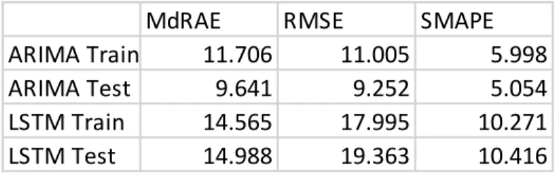
For data with strong seasonality, both models forecast quite effectively. We illustrate this using a popular dataset of Australian beer production. The monthly time series is given in

megaliters, including ale and stout and excluding those with alcoholic content less than 1.15%. Table 1 shows the error measures. Figures 2 and 3 show the visual fit.

MdRAE RMSE SMAPE

ARIMA Train 11.706 11.005 5.998

ARIMA Test 9.641 9.252 5.054

LSTM Train 14.565 17.995 10.271

LSTM Test 14.988 19.363 10.416

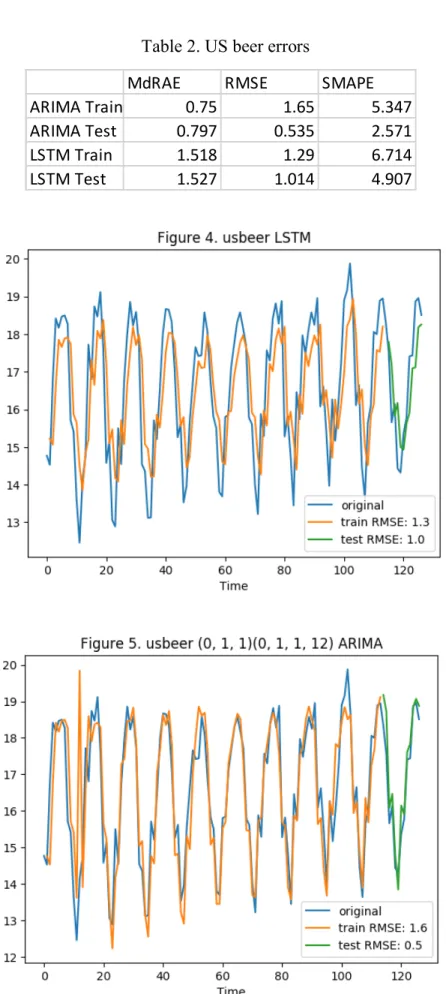
Table 2. US beer errors

MdRAE RMSE SMAPE

ARIMA Train 0.75 1.65 5.347

ARIMA Test 0.797 0.535 2.571

LSTM Train 1.518 1.29 6.714

Another dataset with strong seasonality is the US beer dataset. This contains monthly data for beer production in the US, given in millions of barrels, from January 1983 to July 1993. Table 2 shows the error metrics of the model. Figures 4 and 5 show the visual fit.

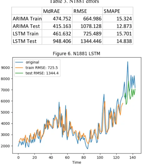
Unfortunately, with little seasonal structure, which is true for most series in the M3 dataset, both models perform poorly. We look at one series from the M3 dataset, N1881. The table and plots below show the fit.

Table 3. N1881 errors

MdRAE RMSE SMAPE

ARIMA Train 474.752 664.986 15.324

ARIMA Test 415.163 1078.128 12.873

LSTM Train 461.632 725.489 15.701

Discussion

The fitting procedure for ARIMA remained consistent for all discussed series. We mainly relied on autocorrelation, partial autocorrelation plots and spectral density to determine the autoregressive and moving average parameters of our model. We first looked at data with strong seasonal structure, the Australian beer data. The ARIMA parameters for this dataset is included in the appendix. Although we expect models to have smaller error for test data, we see that this

is not the case for ARIMA. Across all three error measures (MdRAE, RMSE and SMAPE), the ARIMA model has a smaller test error relative to training error. For example, RMSE test error is 9.252 and train error is 11.005. Although not obvious from figures 2 and 3, the ARIMA model produces a more accurate forecast than the LSTM model, according to all three measures.

We find a nearly identical result for the US beer data. RMSE for the ARIMA model is 9.252, while RMSE for the LSTM model is 19.363. One possible reason for why the LSTM model performs worse can be seen in figure 4. We see that the model tends to underestimate at

the peaks and overestimate at the troughs, preventing it from overfitting to the training set. This is advantageous when past observations are not good indicators of future observations, but in the US beer data, where trends are predictable, this leads to a worse forecast. The ARIMA parameter estimates are included in the appendix.

Many series from the M3 dataset do not have strong seasonal structure like the two above. We looked at one series from the M3 dataset, N1881. We include results for several other series in the appendix. We observe that the models’ predictions tend to lag the actual value by 1 period, suggesting that the best guess given by the model for the next period is usually some weighted average of recent values. Without more information about each series (such as covariates we can use to explain the volatility), the models have difficulty in making accurate forecasts. For some series like that shown in figures 10 and 11, the model fails to capture any significant structure in the data.

Conclusion

We looked at the effectiveness of two methods for making time series forecasts. ARIMA is one of many traditional methods that rely on an underlying stochastic model to extract

information from the data. LSTMs represent an algorithmic approach to analyzing time series data and treats the underlying process as unknown. In order to make our comparison, we used data from various sources including beer data from the US and Australia and anonymized time series from the M3 competition. Our primary evaluation criterion is how well a model performs on out-of-sample data as measured by different error metrics. We concluded that for data with

better. However, data with little to no stucture like those in the M3 are difficult to model, let alone forecast.

Given the sophistication of these models, it may seem surprising how ineffective they are at making accurate forecasts. On the other hand, the amount of information we have at hand to make these forecasts is minimal. Past studies have successfully forecasted complex time series data, but with additional information such as dates, macrotrends and other associated factors. Furthermore, comparing the two methods, LSTM is undoubtedly more complicated and difficult to train and yet it did not surpass the performance of a simple ARIMA model for any of the series. One insight from researchers of the M3 competition is particularly relevant:

“Statistically sophisticated or complex methods do not necessarily provide more accurate forecasts than simpler ones.”

Indeed, LSTMs were not developed for the purpose of analyzing simple time series data like those considered in this paper. It has been the central focus of researchers hoping to solve highly complex tasks, such as generation of text and handwriting. Although other variations of the LSTM may have had more success with the time series data, we believe that for simple settings, traditional methods such as ARIMA that make reasonable assumptions about the underlying structure tend to be more effective.

Appendix • Australian Beer

• US Beer

Statespace Model Results

Dep. Variable: y No. Observations: 428 Model: SARIMAX(7,1,0)x(0,1,1,12) Log Likelihood -1534.6

Date: Wed 02 May 2018 AIC 3087.19 Time: 19:02:02 BIC 3123.722

Sample: 0 HQIC 3101.618 -428 Covariance Type: opg

coef std err z P>|z| ar.L1 -0.9742 0.041 -23.833 0 ar.L2 -1.0125 0.061 -16.634 0 ar.L3 -0.7841 0.077 -10.138 0 ar.L4 -0.721 0.077 -9.396 0 ar.L5 -0.4971 0.071 -6.998 0 ar.L6 -0.1897 0.062 -3.039 0.002 ar.L7 -0.1994 0.041 -4.842 0 ma.S.L12 -0.8154 0.03 -26.982 0 sigma2 91.9102 5.453 16.855 0 Ljung-Box (Q): 88.94 Jarque-Bera (JB): 32.91 Prob(Q): 0 Prob(JB): 0 Heteroskedasticity (H): 4.86 Skew: -0.3 Prob(H) (two-sided): 0 Kurtosis: 4.24

Statespace Model Results

Dep. Variable: y No. Observations: 114 Model: SARIMAX(0,1,1)x(0,1,1,12) Log Likelihood -95.057

Date: Wed 02 May 2018 AIC 196.114

Time: 19:08:52 BIC 204.323

Sample: 0 HQIC 199.446

-114

Covariance Type: opg

coef std err z P>|z| ma.L1 -0.9818 0.074 -13.244 0 ma.S.L12 -0.6134 0.113 -5.42 0 sigma2 0.3475 0.051 6.793 0 Ljung-Box (Q): 99.05 Jarque-Bera (JB): 1.9 Prob(Q): 0 Prob(JB): 0.39 Heteroskedasticity (H): 1.12 Skew: -0.19

• Other M3 Series:

Table 4. N1882 errors

MdRAE RMSE SMAPE

ARIMA Train 49.744 444.588 2.323

ARIMA Test 38.267 41.297 0.384

LSTM Train 38.774 73.041 0.94

MdRAE RMSE SMAPE ARIMA Train 1146.716 1586.388 20.475 ARIMA Test 799.178 1018.651 12.931 LSTM Train 1032.141 1459.496 19.32 LSTM Test 562.753 1275.234 15.297 Table 5. N1886 errors

Bibliography

Back, Andrew and Andreas S. Weigend. 1998. "Discovering Structure in Finance using Independent Component Analysis." Advances in Computational Management Science 2: 309-322.

Cavalcante, Rodolfo C., Rodrigo C. Brasileiro, Victor L. P. Souza, Jarley P. Nobrega, and Adriano L. I. Oliveira. 2016. "Computational Intelligence and Financial Markets: A Survey and Future Directions." Expert Systems with Applications 55: 194-211.

Cho, Kyunghyun, Bart van Merrienboer, Caglar Gulcehre, Dzmitry Bahdanau, Fethi Bougares, Holger Schwenk, and Yoshua Bengio. 2014. “Learning Phrase Representations using RNN Encoder-Decoder for Statistical Machine Translation.” Proceedings of the 2014 Conference on Empirical Methods in Natural Language Processing (EMNLP): 1724–1734.

Dhar, S., T. Mukherjee, and A. K. Ghoshal. 2010. "Performance Evaluation of Neural Network Approach in Financial Prediction: Evidence from Indian Market." IEEE

https://www.scopus.com/inward/record.uri?eid=2-s2.0-79954615790&partnerID=40&md5=c038e5795e3870c931207b42e57519f7.

Hochreiter, Sepp, and Jurgen Schmidhuber. 1997. “Long Short-Term Memory.” Neural Computation 9(8):1735.

Hyndman, Rob J., and Anne B. Koehler. 2005. “Another look at measures of forecast accuracy.”

Kuremoto, Takashi, Shinsuke Kimura, Kunikazu Kobayashi, and Masanao Obayashi. 2014. "Time Series Forecasting using a Deep Belief Network with Restricted Boltzmann Machines." Neurocomputing 137 (Supplement C): 47.

Längkvist, Martin, Lars Karlsson, and Amy Loutfi. 2014. “A Review of Unsupervised Feature Learning and Deep Learning for Time-Series Modeling.” Pattern Recognition Letters 42.

Lu, Chi-Jie, Tian-Shyug Lee, and Chih-Chou Chiu. 2009. “Financial Time Series Forecasting using Independent Component Analysis and Support Vector Regression.” Decision Support Systems 47. doi://doi.org/10.1016/j.dss.2009.02.001.

Majhi, Ritanjali, G. Panda, and G. Sahoo. 2009. “Efficient Prediction of Exchange Rates with Low Complexity Artificial Neural Network Models.” Expert Systems with Applications 36. doi://doi.org/10.1016/j.eswa.

Makridakis, Spyros, and Michele Hibon. 2000. “The M3-Competition: results, conclusions and implications.” International Journal of Forecasting 16: 451–476.

Oliveira, Fagner Andrade de, Luis Enrique Zárate Marcos de Azevedo Reis, and Cristiane Neri Nobre. 2011. “The use of Artificial Neural Networks in the Analysis and Prediction of Stock Prices.” IEEE. doi:10.1109/ICSMC.2011.6083990.

Shen, Furao, Jing Chao, and Jinxi Zhao. 2015. "Forecasting Exchange Rate using Deep Belief Networks and Conjugate Gradient Method." Neurocomputing 167: 243-253.

Tkáč, Michal and Robert Verner. 2016. “Artificial Neural Networks in Business: Two Decades of Research.” Artificial Neural Networks in Business: Two Decades of Research 38. doi://doi.org/10.1016/j.asoc.2015.09.040.

Vedavathi, K., K. Srinivasa Rao, and K. Nirupama Devi. 2014. “Unsupervised Learning

Algorithm for Time Series using Bivariate AR(1) Model.” Expert Systems with Applications Vol. 41. doi://doi.org/10.1016/j.eswa.2013.11.030.