A New Sum-of-Squares Design Framework for Robust Control of Polynomial Fuzzy Systems With Uncertainties

A New Sum-of-Squares Design Framework for

Robust Control of Polynomial Fuzzy Systems

With Uncertainties

著者（英）

Kazuo Tanaka, Motoyasu Tanaka, Ying-Jen Chen,

Hua O. Wang

journal or

publication title

IEEE Transactions on Fuzzy Systems

volume

24

number

1

page range

94-110

year

2016-02

URL

http://id.nii.ac.jp/1438/00009298/

A New Sum-of-Squares Design Framework for

Robust Control of Polynomial Fuzzy Systems with

Uncertainties

Kazuo Tanaka,

Fellow, IEEE,

Motoyasu Tanaka,

Member, IEEE,

Ying-Jen Chen,

Member, IEEE,

and Hua O. Wang,

Senior Member, IEEE

Abstract—This paper presents a new sum-of-squares (SOS, for brevity) design framework for robust control of polynomial fuzzy systems with uncertainties. Two kinds of robust stabilization conditions are derived in terms of SOS. One is global SOS robust stabilization conditions that guarantee the global and asymptotical stability of polynomial fuzzy control systems. The other is semi-global SOS robust stabilization conditions. The latter is available for very complicated systems that are difficult to guarantee the global and asymptotical stability of polynomial fuzzy control systems. The main feature of all the SOS robust stabilization conditions derived in this paper are to be expressed as non-convex formulations with respect to polynomial Lyapunov function parameters and polynomial feedback gains. Since a typical transformation from non-convex SOS design conditions to convex SOS design conditions often results in some conservative issues, the new design framework presented in this paper gives key ideas to avoid the conservative issues. The first key idea is that we directly solve non-convex SOS design conditions without applying the typical transformation. The second key idea is that we bring a so-called copositivity concept. These ideas provide some advantages in addition to relaxations. To solve our SOS robust stabilization conditions efficiently, we introduce a gradient algorithm formulated as a minimizing optimization problem of the upper bound of the time derivative of an SOS polynomial that can be regarded as a candidate of polynomial Lyapunov functions. Three design examples are provided to illustrate the validity and applicability of the proposed design framework. The examples demonstrate advantages of our new SOS design framework for the existing LMI approaches and the existing convex SOS approach.

Index Terms—copositivity, polynomial Lyapunov function, polynomial fuzzy system with uncertainty, robust stabilization, sum of squares.

I. INTRODUCTION

T

Takagi-Sugeno (T-S) fuzzy model-based control [1]. Especially, linear matrix inequalities (LMIs) based designs, e.g., [2], [3], have been paid a lot of attention after LMI-based designs have been discussed in [4]-[6]. A key feature of the approach is that it renders simple, natural and effective design procedures as al-ternatives or supplements to other nonlinear control techniques

Manuscript received April 20, 2007; revised November 18, 2007. This work was supported in part by a Grant-in-Aid for Scientific Research (C) 25420215 from the Ministry of Education, Science and Culture of Japan.

Kazuo Tanaka, Motoyasu Tanaka and Ying-Jen Chen are with the De-partment of Mechanical Engineering and Intelligent Systems, The University of Electro-Communications, Chofu, Tokyo 182-8585 Japan (email: [email protected]; [email protected]; [email protected];).

Hua O. Wang is with the Department of Mechanical Engineering, Boston University, Boston, MA 02215 USA (email: [email protected]).

(e.g., [7]) that require special and rather involved knowledge. The LMI-based design approaches entail obtaining numerical solutions by convex optimization methods such as the interior point method [8].

Though LMI-based approaches have enjoyed great success and popularity, there still exist a large number of design problems that either cannot be represented in terms of LMIs, or the results obtained through LMIs are sometimes conser-vative. Recently, as a post-LMI framework, an SOS based approach has received a great deal of attention in control of nonlinear systems using polynomial fuzzy systems and con-trollers, which includes the well-known Takagi-Sugeno fuzzy systems and controllers as special cases. An SOS approach to polynomial fuzzy control system designs has first presented in [9]-[13]. It can be seen that SOS approaches [9]-[22] provide more extensive and/or relaxed results for the existing LMI approaches [2], [3], [23]-[35] to T-S fuzzy model and control. However, there exists a very few literature on SOS-based robust control designs for polynomial fuzzy systems with uncertainties. To the best of our knowledge, an SOS-based robust control design for polynomial fuzzy systems with uncertainties has been discussed only in [36]. The most important point of SOS-based design conditions is that, to obtain convex SOS design conditions, the existing SOS-based design conditions [9]-[20] utilize a typical transformation from non-convex SOS design conditions to convex SOS design conditions. However, the transformation often results in some conservative issues although no such conservatism exists in LMI transformation cases. In [36], the typical transformation is employed to obtain convex SOS robust stabilization condi-tions. Furthermore, not only the conservative issues but also other two difficulties are found in the existing SOS approach. One is a restrictive polynomial Lyapunov function setting that leads to conservative stability results. The other is that the stability does not generally hold globally in the existing SOS approach. These will be concretely discussed in Remarks 2 and 3. This paper gives new ideas to solve the conservative issues and the difficulties in the existing SOS approach.

This paper presents a new SOS design framework for robust control of polynomial fuzzy systems with uncertainties. The framework gives key ideas to avoid the conservative issues. The first key idea is that we directly solve non-convex SOS design conditions without applying the typical transformation. The second key idea is that we bring a so-called copositivity concept. These ideas provide some advantages in addition to

relaxations. To solve our SOS robust stabilization conditions efficiently, we introduce a gradient algorithm formulated as a minimizing optimization problem of the upper bound of the time derivative of an SOS polynomial that can be regarded as a candidate of polynomial Lyapunov functions.

The rest of the paper is organized as follows. Section II recalls a polynomial fuzzy system defined in [9]-[13] and defines a polynomial fuzzy system with uncertainty. Sections III and IV give a new SOS framework for robust control, i.e., robust stabilization conditions to design a robust fuzzy controller and an algorithm to solve them, respectively. Section V entails two design examples to demonstrate the validity and applicability of the proposed design framework. The examples demonstrate advantages of our SOS robust stabilization condi-tions for the existing LMI approaches and the existing convex SOS approach. Sections VI and VII present semi-global robust stabilization conditions and their design example, respectively. The design example deals with a kind of unmanned aerial vehicles (UAVs) that is a very complicated system with high nonlinearity.

It is assumed that all the matrices and vectors in this paper

have appropriate dimensions. P 0(P 0) means that P

is a positive definite matrix (positive semi-definite matrix).

II. POLYNOMIAL FUZZY SYSTEM WITH UNCERTAINTIES

Consider the following nonlinear system:

˙

x(t) =f(x(t),u(t)), (1) where f is a smooth nonlinear function such that f(0,0) =

0. x(t) = [x₁(t) x₂(t) · · · xn(t)]T is the state vector and

u(t) = [u₁(t) u₂(t) · · · um(t)]T is the input vector. Based on the sector nonlinearity concept [2], we can exactly represent (1) with the following T-S fuzzy model [37] (globally or at least semi-globally).

Model Rule i:

If z₁(t)is Mi1 and· · · and zp(t)is Mip

then x˙(t) =Aix(t) +Biu(t) i= 1,2,· · · , r, (2) where zj(t) (j = 1,2,· · ·, p) is the premise variable. The membership function, Mij, denotes the jth premise variable

component in the ith M odel Rule. r denotes the number

of M odel Rules. Each zj(t) is a measurable time-varying quantity that may be states, measurable external variables and/or time.

The overall dynamics of the system is represented by fuzzy blending of the linear system models. That is, the defuzzification process of the T-S model (2) can be represented as ˙ x(t) = r i=1 wi(z(t)){Aix(t) +Biu(t)} r i=1 wi(z(t)) = r i=1 hi(z(t)){Aix(t) +Biu(t)}, (3) where z(t) = [z1(t)· · ·zp(t)] and wi(z(t)) = p j=1 Mij(zj(t)).

Since the number ofM odel Rule that fire for allt is larger than or equal to one in general, the following relations hold.

r i=1 wi(z(t))>0, wi(z(t))≥0, i= 1,2,· · · , r. Hence, hi(z(t)) = wi(z(t)) r i=1 wi(z(t)) ≥0, r i=1 hi(z(t)) = 1.

In [9] and [12], we proposed a new type of fuzzy model with polynomial model consequence, i.e., fuzzy model whose consequent parts are represented by polynomials. Using the sector nonlinearity concept [2], we exactly represent (1) with the following polynomial fuzzy model (4) even if the nonlinear system (1) contains polynomial elements. The main difference between the T-S fuzzy model [37] and the polynomial fuzzy model is consequent part representation. The fuzzy model (4) has a polynomial model consequence.

Model Rule i:

If z₁(t)is Mi1 and· · · and zp(t)is Mip

thenx˙(t) =Ai(x(t))ˆx(x(t)) +Bi(x(t))u(t), (4) wherei= 1,2,· · ·, r.rdenotes the number ofM odel Rules.

ˆ

x(x(t))is a column vector whose entries are all monomials in x(t). That is, xˆ(x(t)) ∈ RN _{is an N ×1 vector of} monomials inx(t). A monomial in x(t)is a function of the formxα1

1 xα22· · ·xαnn, whereα1,α2,· · ·,αn are nonnegative integers. Ai(x(t)) ∈ Rn×N and Bi(x(t)) ∈ Rn×m are polynomial matrices in x(t). Therefore, Ai(x(t))ˆx(x(t)) +

Bi(x(t))u(t) is a polynomial vector. Thus, the polynomial fuzzy model (4) has a polynomial in each consequent part. We assume that

ˆ

x(x(t)) = 0 iffx(t) = 0 throughout this paper.

The defuzzification process of the model (4) can be repre-sented as ˙ x(t) = r i=1 hi(z(t)){Ai(x(t))ˆx(x(t)) +Bi(x(t))u(t)}. (5) The polynomial fuzzy model is an extension of the T-S fuzzy model. The extension bring us some advantages [12]. One is that SOS stabilization conditions provides more relaxed results than the existing LMI stabilization conditions. Another advance is that original nonlinear systems with polynomial terms can be exactly and globally represented by polynomial fuzzy models although the T-S fuzzy models are sometimes not global models for the original nonlinear systems with polynomial terms.

Remark 1. Stability conditions for the T-S fuzzy system have been mainly represented in terms of LMIs [2]. Hence, the LMI stability conditions can be solved numerically and efficiently by interior point algorithms, e.g., by LMI solvers. On the other hand, the convex SOS conditions in [9]-[20], [36] for polynomial fuzzy systems are represented as convex SOS problems. Clearly, the problems can not be directly solved by LMI solvers, but they can be solved via an SOS solver (SOSOPT [38], SOSTOOLS [39], etc.) and an SDP solver [40], [41].

This paper focuses on stabilization of the polynomial fuzzy model with uncertainties. Hence, we define a polynomial fuzzy model with uncertainties as follows.

Model Rule i: If z₁(t)is Mi1 and· · · and zp(t)is Mip then ˙ x(t) ={Ai(x(t)) +Dai(x(t))Δai(x(t))Eai(x(t))}xˆ(x(t)) +{Bi(x(t)) +Dbi(x(t))Δbi(x(t))Ebi(x(t))}u(t), (6) where i= 1,2,· · ·, r. Dai(x(t)), Dbi(x(t)),Eai(x(t))and

Ebi(x(t))are polynomial matrices inx(x(t)).Δai(x(t))and

Δbi(x(t))denote uncertain matices inx(t)and satisfy

Δai(x(t))≤βai(x(t)), (7)

Δbi(x(t))≤βbi(x(t)), (8) where βai(x(t))andβbi(x(t))denote the upper bound of the norm of the uncertainties.

The defuzzification process of the model (6) can be repre-sented as ˙ x(t) = r i=1 hi(z(t)){Ai(x(t))ˆx(x(t)) +Bi(x(t))u(t) +Dai(x(t))Δai(x(t))Eai(x(t))ˆx(x(t)) +Dbi(x(t))Δbi(x(t))Ebi(x(t)))u(t)}. (9) From now, to lighten the notation, we will drop the notation with respect to time t. For instance, we will employ x and

ˆ

x(x)instead ofx(t)andxˆ(x(t)), respectively. Thus, we drop the notation with respect to time t, but it should be kept in mind that xandxˆ(x)means x(t)andxˆ(x(t)), respectively. For the model (9), we design the following fuzzy controller.

u = −

r

i=1

hi(z)Fi(x)ˆx(x) (10) A convex SOS robust design condition for the control system consisting of (9) and (10) was presented in [36]. However, as will be mentioned in Remarks 2 and 3, some disadvantages exist in the existing SOS approaches [9]-[20] [36].

Remark 2. In [9]-[20] and [36], the Lyapunov function candidate (11) is used.

V(x) = ˆxT(x)X−1(˜x)ˆx(x), (11)

where _X(˜_x) is a polynomial matrix in _x˜. If_xˆ(_x) =_x and X−1(˜x)is a constant matrix, then (11) reduces to the quadrat-ic Lyapunov function. The zero equilibrium is asymptotquadrat-ically stable when the Lyapunov function exists. However, the glob-ality is not guaranteed. The stability holds globally only if X−1(˜x)is a constant matrix. The important point is that, to avoid introducing non-convex condition, _x˜ in the polynomial matrix_X(˜_x)is defined as follows. Let_K={k1, k2,· · ·, km}

denote the row indices of_Bi(x)whose corresponding row is

equal to zero, and define_x˜ = (xk1, xk2,· · ·, xkm)using the K. In other words, to avoid introducing non-convex condition, it is assumed in the literature that X(˜x) only depends on states_x˜whose dynamics is not directly affected by the control input, namely states whose corresponding rows in _Bi(_x)are zero. The restriction caused by _x˜ depends on the _Bi(_x) matrices and it leads to some conservative stability results. A new SOS framework that will be presented in Section III permits a non-restrictive polynomial Lyapunov function setting.

Remark 3. As mentioned in Remark 2, (11) is employed as a candidate Lyapunov function. The transformation from non-convex conditions to convex conditions is carried out as follows. The time derivative ofV(x)along the feedback system trajectory, that consists of (5) and (10), can be represented by the general form.

˙

V(x) = ˆxT(x)S(x)ˆx(x)<0, (12)

where _S(_x) is a non-convex polynomial matrix since it has cross terms with respect to_X−1(˜_x)and_Fi(_x). The transfor-mation is carried out by dropping_xˆ(_x)off from both side of the inequality and by multiplying the dropped inequality on the left and right by_X(˜_x). As a result of the transformation, we have the following convex condition with respect to_X(˜_x) and _Mi(x), whereMi(x) =Fi(x)X(˜x).

−X(˜x)S(x)X(˜x)0.

Finally, we arrive at the convex SOS condition, −vT_{X(˜

x)S(x)X(˜x) +(x)I}v is SOS,

where(x)is a slack variable (a radially unbounded positive definite polynomial) to keep the positivity of the SOS condition. In the transformation, we utilize the fact that−S(_x)0⇒ −xˆT(x)S(x)ˆx(x) > 0. However, it should be emphasized that this is a sufficient condition, i.e., in general, it is not always satisfied that−xˆT_{(x)S(x)ˆx(x)>0⇒ −S(x)0.}

It becomes a necessary and sufficient condition only if _S(_x) is a constant matrix and _xˆ(_x) = _x. Only in the case, no conservatism exists. In the LMI case [2], this path is always equivalent since _S(_x) is a constant matrix and _xˆ(_x) = _x. Thus, this conservative path in the convex SOS transformation often causes conservative results although this path is always equivalent in the LMI case. In [36], the same transformation is employed to obtain convex SOS robust stabilization conditions. A new SOS framework that will be presented in Section III can avoid this main problem.

A new SOS framework that will be presented in Section III can completely avoid the two problems mentioned in Remarks

2 and 3. The utility of the new SOS design framework will be demonstrated in design examples.

III. SOS STABILIZATIONCONDITIONS

Section III presents SOS stabilization conditions based on copositivity concept.

If (13) holds, the matrix J = [Jij]∈R× is copositive.

yTJy= i=1 j=1 yiyjJij ≥0, (13) where y= [y₁, y₂, . . . , y]T ∈Randyi≥0. Since checking copositivity of a matrix is a co-NP complete problem, we take a technique for copositivity checking relaxation [39].

Corollary 1. [39]

A relaxation is to introduce yi = ˆyi2 and to check whether

(14) is satisfied or not. Qs(ˆy) = ( k=1 ˆ y_k2)s i=1 j=1 ˆ y2_iyˆ_j2Jij is SOS, (14)

where yˆ= [ˆy₁,yˆ₂, . . . ,yˆ]T and sis a nonnegative integer. By using the copositivity checking relaxation, we derive SOS robust stabilization conditions that are different from the SOS robust stabilization conditions in [36]. Theorem 1 presents the SOS robust stabilization conditions.

Theorem 1. If there exist a polynomial V(x), polynomial matrices_Fj(x)and polynomialsg¯ij(x)such that (15)∼(17)

are satisfied with α < 0 and λ > 0, the polynomial fuzzy controller (10) stabilizes the system (9), andV(x)becomes a Lyapunov function. V(x)−(x) is SOS, (15) ( r k=1 ˆ h2_k)s r i=1 r j=1 ˆ h2_iˆh2_j{−¯Λij(x) +αV(x)} is SOS, (16) v₁TLij(λ,x)v1 is SOS, (17)

where _v1 denotes vector that is independent of_x. (x) is a radially unbounded positive definite polynomial and s is a non-negative integer. ¯Λij(x) = ∂V(x) ∂x {Ai(x)−Bi(x)Fj(x)}xˆ(x) +¯gij(x), (18) Lij(λ,x) = ⎡ ⎢ ⎢ ⎢ ⎢ ⎣ λg¯ij(x) ∗ ∗ ∗ ∗ λDT ai(x)( ∂V(x) ∂x )T 2I 0 0 0 λDT bi(x)( ∂V(x) ∂x ) T _{0 2I 0 0} βai(x)Eai(x)ˆx(x) 0 0 2I 0 βbi(x)Ebi(x)Fj(x)ˆx(x) 0 0 0 2I ⎤ ⎥ ⎥ ⎥ ⎥ ⎦. (19)

The asterisk ∗ denotes the transposed elements (matrices) for symmetric positions.

Proof:

Consider a candidate of Lyapunov functionsV(x). The time derivative ofV(x)is given as

˙

V(x) = ∂V(x)

∂x x˙. (20)

By subsitituting the closed loop dynamics consisting of (9) and (10) into (20), the time derivative ofV(x)along the trajectory becomes ˙ V(x) = r i=1 r j=1 hihj ∂V(x) ∂x {Ai(x)−Bi(x)Fj(x) +Dai(x)Δai(x)Eai(x) −Dbi(x)Δbi(x)Ebi(x)Fj(x)}xˆ(x) = r i=1 r j=1 hihj{ ∂V(x) ∂x (Ai(x) −Bi(x)Fj(x))ˆx(x) +ζi(x)ηij(x)}, where ζi(x) = ∂V(x) ∂x Dai(x) ∂V(x) ∂x Dbi(x) , ηij(x) = Δai(x)Eai(x)ˆx(x) −Δbi(x)Ebi(x)Fj(x)ˆx(x) . Note that λζi(x)ζiT(x) + 1 λη T ij(x)ηij(x) ≥ ζi(x)ηij(x) +ηTij(x)ζiT(x) for anyλ >0. In addition, sinceζi(x)ηij(x) =ηijT(x)ζiT(x), we have the following relation.

λζi(x)ζiT(x) + 1 λη T ij(x)ηij(x)≥2ζi(x)ηij(x). Hence ζi(x)ηij(x) ≤ λ₂ζi(x)ζiT(x) + 1 2λη T ij(x)ηij(x) = λ₂∂V(x) ∂x Dai(x)D T ai(x)( ∂V(x) ∂x ) T + λ₂∂V(x) ∂x Dbi(x)D T bi(x)( ∂V(x) ∂x ) T + ₂1 λxˆ T₍ x)EaiT(x)ΔTai(x)Δai(x)Eai(x)ˆx(x) + ₂1 λxˆ T₍ x)FjT(x)EbiT(x)ΔTbi(x) ×Δbi(x)Ebi(x)Fj(x)ˆx(x) ≤ Πij(λ,x), where Πij(λ,x) = λ 2 ∂V(x) ∂x Dai(x)D T ai(x)( ∂V(x) ∂x ) T + λ 2 ∂V(x) ∂x Dbi(x)D T bi(x)( ∂V(x) ∂x ) T + ₂1 λβ 2 ai(x)ˆxT(x)EaiT(x)Eai(x)ˆx(x) + 1 2λβ 2 bi(x)ˆxT(x)FjT(x)EbiT(x)Ebi(x)Fj(x)ˆx(x).

From the above inequality, we have ˙ V(x) = r i=1 r j=1 hihj{ ∂V(x) ∂x (Ai(x) −Bi(x)Fj(x))ˆx(x) +ζi(x)ηij(x)} ≤ r i=1 r j=1 hihj{ ∂V(x) ∂x (Ai(x) −Bi(x)Fj(x))ˆx(x) +Πij(λ,x)}. We introduce a polynomial g¯ij(x)satisfying

r i=1 r j=1 hihjΠij(λ,x)≤ r i=1 r j=1 hihjg¯ij(x). (21) Then, we have ˙ V(x) ≤ r i=1 r j=1 hihj{ ∂V(x) ∂x (Ai(x) −Bi(x)Fj(x))ˆx(x) + ¯gij(x)}. (22) To show that V˙(x)<0 atx= 0, we consider the condition satisfying V˙(x)≤αV(x), where α <0. That is,

r i=1 r j=1 hihj{ ∂V(x) ∂x (Ai(x)−Bi(x)Fj(x))ˆx(x) +¯gij(x)} −αV(x)≤0.

By applying the copositivity presented in Lemma 1, we obtain (16).

On the other hand, from the inequality (21) and λ >0, we obtain r i=1 r j=1 hihj{λg¯ij(x)−λΠij(λ,x)} ≥0. (23) Using schur complement, (23) can be converted to

r i=1 r j=1 hihjLij(λ,x)≥0, (24) where Lij(λ,x) = ⎡ ⎢ ⎢ ⎢ ⎢ ⎣ λ¯gij(x) ∗ ∗ ∗ ∗ λDTai(x)( ∂V(x) ∂x ) T ₂ I 0 0 0 λDT bi(x)( ∂V(x) ∂x )T 0 2I 0 0 βai(x)Eai(x)ˆx(x) 0 0 2I 0 βbi(x)Ebi(x)Fj(x)ˆx(x) 0 0 0 2I ⎤ ⎥ ⎥ ⎥ ⎥ ⎦.

The condition (24) holds if (17) is satisfied.

Theorem 2. Assume that Δbi(x) = 0 for all i, i.e., there

are no uncertainties with respect to the input terms. Then, the SOS robust stabilization conditions in Theorem 1 become simple. If there exist a polynomial function V(x), polynomial matrices _Fj(x)and polynomials¯gi(x)such that (25)∼(27)

are satisfied with α < 0 and λ > 0, the polynomial fuzzy controller (10) stabilizes the system (9).

V(x)−(x) is SOS, (25) ( r k=1 ˆ h2_k)s r i=1 r j=1 ˆ h2_iˆh2_j{−¯Λij(x) +αV(x)} is SOS, (26) vT1 ⎡ ⎣ _λDTλg¯i(x) ∗ ∗ ai(x)( ∂V(x) ∂x ) T ₂ I 0 βai(x)Eai(x)ˆx(x) 0 2I ⎤ ⎦_v1 is SOS, (27)

where (x) is a radially unbounded positive definite polyno-mial,s is a non-negative integer, and

¯Λij(x) = ∂V(x)

∂x {Ai(x)−Bi(x)Fj(x)}xˆ(x)

+¯gi(x). (28)

Proof: The proof is omitted since it is directly obtained from Theorem 1. In this case, (17) is reduced to (27).

IV. ALGORITHM TOSOLVESOS CONDITIONS

Section IV presents an algorithm to solve the SOS robust stabilization conditions given in Section III. The algorithm is based on a gradient algorithm formulated as a minimizing optimization problem of the upper bound of the time derivative of an SOS polynomial that can be regarded as a candidate of polynomial Lyapunov functions.

We first explain the outline of its key idea below.

A. Key Idea

Consider the non-convex condition

φg(x)φh(x)≺0, (29) where φg(x) and φh(x) are polynomial matrices in x and both of them are decision variables (matrices). The problem is to find a solution satisfying (29). With a positive definite

polynomial matrix ψ(x) in x, the problem (29) may be

converted as

−φg(x)φh(x) +αψ(x)0. (30) If we get a solution of (30) withα <0, the problem (29) is feasible. Regularly, (30) can be converted as

‘−vT{φg(x)φh(x)−αψ(x)}v is SOS’,

where v denotes a vector that is independent of x. Note that the SOS condition is bilinear (not convex) with respect to de-cision variables since there exists the termφg(x)φh(x). Now consider very small perturbationsδφg(x),δφh(x)andδψ(x) as in [42], [43]. Since δφg(x) and δφh(x) are very small perturbations, it can be noted with a reasonable approximation that

φg(x)φh(x) (φg(x) +δφg(x))(φh(x) +δφh(x))

= φg(x)φh(x) +δφg(x)φh(x)

+φg(x)δφh(x) +δφg(x)δφh(x). Note that the term, δφg(x)δφh(x), is an extremely small in comparison with other terms since it is the product term of these small perturbations. Then, (φg(x) +δφg(x))(φh(x) + δφh(x))can be represented asφg(x)φh(x)+δφg(x)φh(x)+ φg(x)δφh(x). From this fact, we transform

‘−φg(x)φh(x) +αψ(x)0’ to

‘−vT{φg(x)φh(x) +δφg(x)φh(x) +φg(x)δφh(x)

−αψ(x)−αδψ(x)}v is SOS. (31) Now we can formulate (31) as a minimizing optimization problem based on convex SOS with respect toδφg(x),δφh(x) andδψ(x). min δφg(x),δφh(x),δψ(x)α subject to vT1{ψ(x) +δψ(x)−(x)}v1 is SOS, (32) −vT 2{φg(x)φh(x) +δφg(x)φh(x) +φg(x)δφh(x) −αψ(x)−αδψ(x)}v2 is SOS, (33) vT3 GφTg(x)φg(x) δφg(x) δφg(x) I v3 is SOS, (34) vT4 HφTh(x)φh(x) δφh(x) δφh(x) I v4 is SOS, (35) vT5 ψψT(x)ψ(x) δψ(x) δψ(x) I v5 is SOS, (36) where v1 - v5 denote vectors that are independent of x.G, H and ψ are very small positive values. (x) is a radially unbounded positive definite polynomial. (34), (35) and (36) guarantee to keep the assumption that δφg(x), δφh(x) and δψ(x)are very small perturbations, respectively.

Note that the decision variables are δφg(x), δφh(x) and δψ(x)in the minimizing optimization. The minimizing opti-mization is iteratively performed by substituting the solutions

δφg(x),δφh(x)andδψ(x)

obtained at the Nth iteration into the iteration law φNg+1(x) =φgN(x) +δφg(x), φN_h+1(x) =φ_hN(x) +δφh(x), ψN+1(x) =ψN(x) +δψ(x).

Thus, the decision variables are updated so as to minimize the minimizing parameter α. As a result, φg(x), φh(x) and ψ(x) are iteratively updated from the initial setting (φ0_g(x), φ0_h(x)andψ0(x)) so as to minimize the minimizing parameter α. The initial setting of φ0_g(x) φ_h0(x) and ψ0(x) should be sometimes carefully selected. So the grid search will be employed to select the initial setting. If the minimizing optimization problem is feasible with α < 0, it is a solution of (29), i.e.,φg(x)φh(x)≺0.

B. Algorithm

We can consider

V(x) = ¯xT(x)Px¯(x),

whereP ∈Rρ×ρ is a positive definite matrix andx¯(x)∈Rρ

is a column vecrtor whose entries are all monomials inxsuch thatx¯(x) =0iffx=0and||x¯(x)|| → ∞for||x(x)|| → ∞. For example, if we choose the vector x¯(x) = [x₁ x₂]in the case of x = [x₁ x₂], V(x) becomes a quadratic Lyapunov

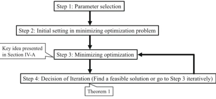
Step 2: Initial setting in minimizing optimization problem

Step 3: Minimizing optimization

Step 4: Decision of Iteration (Find a feasible solution or go to Step 3 iteratively) Key idea presented

in Section IV-A

Theorem 1 Step 1: Parameter selection

Fig. 1. Outline of algorithm.

function. Ifx¯(x) = [x2₁ x₁x₂ x2₂]is chosen, V(x)becomes a 4th-order polynomial Lyapunov function.

The algorithm to solve the SOS conditions consists of four steps. Fig. 1 shows the outline of the algorithm. The key idea mentioned in Section IV-A will be used in Step 3. We check whether the SOS conditions given in Theorem 1 are strictly and exactly feasible or not in Step 4. This algorithm can be regarded as a gradient algorithm formulated as a minimizing optimization problem of the upper bound of the time derivative of the polynomial V(x). Table I summarizes main variables and parameters in the minimizing optimization algorithm, wherepiis thei-th diagonal element of the positive definite matrixP. For simplicity, all the non-diagonal elements of the positive definite matrixP are set to zero in the initial setting. However, note that, after performing the algorithm, the

nondiagonal elements of the matrixP can become non-zero.

In fact, the complicated example in Section VII obtains the matrixP whose nondiagonal elements are non-zero although the nondiagonal elements of the matrix P are set to zero in the initial setting.

TABLE I

LIST OF MAIN VARIABLES AND PARAMETERS IN MINIMIZING OPTIMIZATION ALGORITHM.

N number of iteration

λmin_,λmax _{lower and upper bounds ofλ}

satisfying0< λmin≤λ≤λmax

pmin

i ,pmaxi lower and upper bounds ofpi

satisfying0< pmin_i ≤p_i≤pmax_i

qλ,Δλ number of divided segments and interval such thatq_λΔλ=λmax−λmin

qpi,Δp_i number of divided segments and intervals such thatqpiΔpi=pmaxi −pmini

Step 1: SetN = 0. Select positive scalarsλmin,λmax,Δλ and Δpi (i = 1,2,· · ·ρ) satisfying the relations defined in Table I.

Step 2: For all the combinations (λ, p₁, p₂,· · ·, pρ) on all the grid points[λmin_λmax_]×[pmin

1 pmax2 ]×· · ·×[pminρ pmaxρ ] with the intervals Δλ,Δp₁,Δp₂,· · · Δpρ, solve

min

Fj(x),¯gij(x)

α subject to(15),(16)and(17) (37) and find the grid point with the minimum α. If a grid point withα <0is found, it is a strict solution of Theorem 1. If any feasible solutions withα <0are not obtained, then substitute

point into FN

j (x),¯gNij(x),VN(x) andλN, respectively, and go to Step 3.

Step 3: Set Fj(x) = FjN(x), ¯gij(x) = ¯gNij(x), V(x) = VN(x)andλ=λN. For the givenFj(x),¯gij(x),V(x), and λ, solve the following SOS optimization problem.

min

δFj(x),δV(x),δ¯gij(x),δλα subject to(38)∼(44) The SOS conditions (38) ∼(44) are derived by applying the key idea to Theorem 1.

V(x) +δV(x)−(x) is SOS, (38) ( r k=1 ˆ h2_k)s r i=1 r j=1 ˆ h2_iˆh2_j{−(¯Λij(x) +δ¯Λij(x)) +α(δV(x) +V(x))} is SOS, (39) ( r k=1 ˆ h2_k)s r i=1 r j=1 ˆ h2_iˆh2_j × v1T ⎡ ⎢ ⎢ ⎢ ⎢ ⎣ λ¯gij(x) +δλg¯ij(x) +λδg¯ij(x) DT ai(x)μT(x) DT bi(x)μT(x) βai(x)Eai(x)ˆx(x) βbi(x)Ebi(x)(Fj(x) +δFj(x))ˆx(x) ∗ ∗ ∗ ∗ 2I 0 0 0 0 2I 0 0 0 0 2I 0 0 0 0 2I ⎤ ⎥ ⎥ ⎥ ⎥ ⎦v1 is SOS, (40) v₂T VV2(x) δV(x) δV(x) I v2 is SOS, (41) v₃T FFjT(x)Fj(x) δFj(x) δFT j (x) I v3 is SOS,(42) v4T gg¯ij2(x) δg¯ij(x) δg¯ij(x) I v4 is SOS, (43) v₅T Lλ2 δλ δλ I v5 is SOS, (44) where δ¯Λij(x) = ∂δV(x) ∂x {Ai(x)−Bi(x)Fj(x)}xˆ(x) −∂V(x) ∂x Bi(x)δFj(x)ˆx(x) +δg¯ij(x), μ(x) = λ(∂V(x) ∂x ) +δλ( ∂V(x) ∂x ) +λ( ∂δV(x) ∂x ). v1 - v5 denote vectors that are independent of x.V,F,g andL are very small positive values andsis a non-negative integer.

Step 4: For δV(x) and δλ obtained by solving the SOS optimization problem in Step 3, let VN+1_{(x) = V}N_{(x) +} δV(x) and λN+1 _{= λ}N _{+δλ, respectively. Then set N =} N+ 1. Next, set V(x) =VN_(x)andλ=λN_{. For the given} V(x)andλ, solving the minimizing SOS problem (45).

min

Fj(x),g¯ij(x)

α subject to(15),(16)and(17) (45) If a feasible solution with α < 0 is obtained, it is a strict solution of Theorem 1. If any feasible solutions with α <0

are not obtained, then substitute Fj(x) and ¯gij(x) obtained by solving (45) intoFN

j (x)and¯gNij(x), respectively, and go to Step 3.

Remark 4. Assume thatΔbi(x) =0for alli, i.e., there are

no uncertainties with respect to the input terms. Then, (40) and (43) can be simplified as (46) and (47), respectively.

( r k=1 ˆ h2k)s r i=1 r j=1 ˆ h2iˆh2j× vT1 ⎡ ⎣ λg¯i(x) +_DTδλg¯i(x) +λδ¯gi(x) ai(x)μT(x) βai(x)Eai(x)ˆx(x) ∗ ∗ 2I 0 0 2I ⎤ ⎦_v1 is SOS, (46) vT4 gg¯2i(x) δg¯i(x) δ¯gi(x) I v4 is SOS. (47)

Remark 5. We need to carefully deal with SOS solutions since some numerical reliability options exist in the SOS solvers and their feasible results might be changed very slightly according to the options, particularly, for complicated systems. In other words, feasible area plots (, e.g., such as Figs. 4 and 5) might change very slightly according to the options. To obtain more reliable solutions for SOS conditions, we perform the following double checking throughout this paper. After getting a feasible solution in the algorithm, we carefully perform the so-called SOS test (, e.g., ’issos’ command in SOSOPT) for the polynomials calculated by substituting the feasible solution into the considered SOS conditions. That is, with one of most reliable options, we check whether the polynomials (calculated by substituting the feasible solution into the considered SOS conditions) are judged as SOS polynomials or not. If the check returns an infeasible result, we strictly judge ‘infeasible’. This double checking is important to have reliable solutions in the use of SOSOPT[38] or SOSTOOLS [39] and an SDP solver [40], [41]

V. DESIGNEXAMPLES

A. Design Example I

Consider the following nonlinear system with an uncertain-ty. ˙ x₁= (−1 + Δ(t) +x₁+x₁2+x₁x₂−x2₂)x₁ +x₂+x₁u, ˙ x₂=−2 sin(x₁)−6x₂+ 7u, (48) where Δ(t) is the uncertainty satisfying |Δ(t)| ≤ c for all t. All the simulation results given in this design example are carried out for Δ(t) = csin(200πt). However, it should be noted thatΔ(t)is the uncertain term and only its upper bound, i.e.c, is known as well as the standard robust control setting. Using the sector nonlinearity technique [2], the nonlinear system with the uncertainty is exactly converted into the fol-lowing two-rule polynomial fuzzy system with uncertainties:

˙ x= r i=1 hi(z){(Ai(x) +Dai(x)Δai(x)Eai(x))x +Bi(x)u)},

where r=2,xˆ(x) =x= [x₁, x₂],z=x₁, and A1(x) = −1 +x₁+x2₁+x₁x₂−x2₂ 1 −2 −6 , A2(x) = −1 +x₁+x2₁+x₁x₂−x2₂ 1 0.4344 −6 , B1(x) =B2(x) = x₁ 7 , Da1(x) =Da2(x) = c 0 , Δa1(x) =Δa2(x) = Δ(t)/c, Ea1(x) =Ea2(x) = 1 0 , h1(z) =sin(x₁1) + 0.2172x1 .2172x₁ , h2(z) = x₁−sin(x₁) 1.2172x₁ . Since ||Δa1(x)|| =||Δa2(x)|| =||Δ(t)/c|| ≤1, we have βa1=βa2= 1. Moreover, the algorithm presented in Section IV is carried out with the initial setting s = 0, g = 0.001, F = 0.001, V = 0.001, L = 0.001, λmin = 0.2, λmax _{= 5, Δλ = 0.8, p}min

i = 0.2, pmaxi = 1, Δpi = 0.2 for i = 1,2. To show the validity of derived conditions, we compare the feasible values of c for the proposed robust control design method and the SOS-based design method of [36]. The proposed robust control design method is feasible forc≤0.76, and the method of [36] is feasible forc≤0.39. It shows that the proposed robust design method provides more relaxed results than the method of [36].

TABLE II FEASIBLE AREAS FORc. Convex SOS robust [36] c≤0.39 Our SOS robust c≤0.76

For c = 0.76, Fig. 2 shows the behavior of the nonlinear system (48) with u= 0. Thus, the system is unstable when u = 0. By solving the conditions in Theorem 2, a feasible solution forc= 0.76 can be obtained as

λ= 0.6811, V(x) = 1.0524x2₁+ 0.1361x2₂ F₁(x) = 1.6566x1+ 0.2669x2+ 0.8952 0.2669x₁−0.1902 T , F₂(x) = 1.6314x₁+ 0.2696x₂+ 1.0418 0.2696x₁−0.2061 T , ¯ g₁(x) = 0.6850x4₁−0.5481x3₁x₂+ 1.1416x2₁x2₂ −0.0932x3₁+ 1.4081x2₁x₂+ 0.5751x₁x2₂ + 1.8407x2₁+ 0.0615x1x2+ 0.6297x2₂, ¯ g₂(x) = 0.6797x4₁−0.5397x3₁x₂+ 1.1377x2₁x2₂ + 0.0217x3₁+ 1.3704x₁2x₂+ 0.5679x₁x2₂ + 1.8395x2₁−0.0914x₁x₂+ 0.6296x2₂.

Fig. 3 shows the controlled behavior for six different initial conditions. It can be seen from Fig. 3 that the design fuzzy controller stabilizes the system from all the initial conditions although the system has uncertainties.

−10 −8 −6 −4 −2 0 2 4 6 8 10 −10 −8 −6 −4 −2 0 2 4 6 8 10 x 1 x2

Fig. 2. Behavior of the nonlinear system (48) withu= 0.

−10 −8 −6 −4 −2 0 2 4 6 8 10 −10 −8 −6 −4 −2 0 2 4 6 8 10 x₁ x2

Fig. 3. Controlled behavior of the nonlinear system (48).

Based on the sector nonlinearity technique [2], the nonlinear system (48) can be exactly represented by a T-S fuzzy model for x₁ ∈[−d₁ d₁] andx₂ ∈[−d₂ d₂], where d₁ and d₂ are constant satisfying 0 < d₁ <∞and 0 < d₂ <∞. The T-S fuzzy model is obtained as

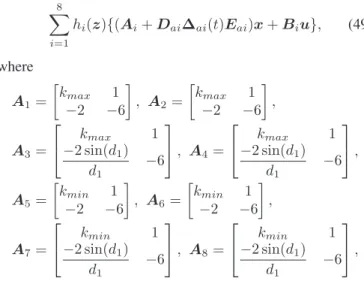
8 i=1 hi(z){(Ai+DaiΔai(t)Eai)x+Biu}, (49) where A1= kmax 1 −2 −6 , A2= kmax 1 −2 −6 , A3= ⎡ ⎣−2 sin(kmaxd₁) 1 d₁ −6 ⎤ ⎦, A4= ⎡ ⎣−2 sin(kmaxd₁) 1 d₁ −6 ⎤ ⎦, A5= kmin 1 −2 −6 , A6= kmin 1 −2 −6 , A7= ⎡ ⎣_{−2 sin(}kmind1) 1 d₁ −6 ⎤ ⎦, A8= ⎡ ⎣_{−2 sin(}kmind1) 1 d₁ −6 ⎤ ⎦,

0 0.5 1 1.5 0 1 2 3 4 5 6 7 8 9 10 d 1 d 2

Fig. 4. Feasible area of the LMI-based robust control design conditions proposed in [2] for the T-S fuzzy model (49) withc= 0.76.

B1=B3=B5=B7= d₁ 7 , B2=B4=B6=B8= −d₁ 7 , Dai= c 0 , i= 1, · · ·,8, Δai= Δ(t)/c, i= 1, · · ·,8, Eai= 1 0, i= 1, · · · ,8, kmax= max |x1|<d1,|x2|<d2(−1 + x₁+x2₁+x₁x₂−x2₂), kmin = min |x1|<d1,|x2|<d2(−1 + x₁+x2₁+x₁x₂−x2₂). The membership functions are given as follows.

h₁(z) = k−kmin kmax−kmin .sinx1−(sind1/d1)x1 (1−(sind₁/d₁))x₁ . x1+d1 2d₁ h2(z) = k−kmin kmax−kmin .sinx1−(sind1/d1)x1 (1−(sind₁/d₁))x₁ . d₁−x₁ 2d₁ h₃(z) = k−kmin kmax−kmin . x1−sinx1 (1−(sind₁/d₁))x₁. x₁+d₁ 2d₁ h₄(z) = k−kmin kmax−kmin . x1−sinx1 (1−(sind₁/d₁))x₁. d₁−x₁ 2d₁ h₅(z) = kmax−k kmax−kmin .sinx1−(sind1/d1)x1 (1−(sind₁/d₁))x₁ . x₁+d₁ 2d₁ h₆(z) = kmax−k kmax−kmin .sinx1−(sind1/d1)x1 (1−(sind₁/d₁))x₁ . d₁−x₁ 2d₁ h₇(z) = kmax−k kmax−kmin . x1−sinx1 (1−(sind₁/d₁))x₁. x₁+d₁ 2d₁ h₈(z) = kmax−k kmax−kmin . x1−sinx1 (1−(sind₁/d₁))x₁. d₁−x₁ 2d₁ Fig. 4 shows the feasible area of the LMI-based robust control design conditions proposed in [2] for the T-S fuzzy model (49) with c= 0.76.

Remark 6. For nonlinear systems with polynomial terms, it is impossible to exactly construct a global T-S fuzzy model. In this example, a local T-S fuzzy model with 8 rules can

be constructed by assuming the ranges of x₁ and x₂, e.g., |x₁| < d₁ and |x₂| < d₂, where d₁ and d₂ are nonnegative values. If we select huge values for d₁ and d₂, the local T-S fuzzy model could be a global model, however, it becomes much harder to guarantee the stability for larger values ofd₁

andd₂. In other words, smaller values ofd₁and d₂ becomes easier to guarantee the stability of the local T-S fuzzy model. However, the LMI robust conditions for T-S fuzzy models are infeasible even for very small values, e.g., d1 > 0.96 when

c= 0.76.

B. Design example II

Consider the following nonlinear system with uncertainties.

˙ x₁= (−1 + Δa(t) +x1+x21+x1x2−x22)x1 +x₂+x₁u, ˙ x₂=−2 sin(x₁)x₁−6x₂−4 sin(x₁)(1 + Δb(t))u, (50) where Δa(t) and Δb(t) are the uncertainties satisfying

|Δa(t)| ≤ ca and |Δb(t)| ≤ cb for all t. All the simulation results given in this design example are carried out for

Δa(t) =casin(200πt) andΔb(t) =cbsin(200πt). However, it should be noted thatΔa(t)andΔb(t)are the uncertain terms and only their upper bounds, i.e.ca andcb, are known as well as the standard robust control setting.

Using the sector nonlinearity technique [2], the nonlinear system with the uncertainties is exactly converted into the polynomial fuzzy system (9) withr=2,xˆ(x) =x= [x1, x2],

z=x₁ and A1(x) = −1 +x₁+x2₁+x₁x₂−x2₂ 1 −2 −6 , A2(x) = −1 +x₁+x2₁+x₁x₂−x2₂ 1 2 −6 , B1(x) = x₁ −4 , B2(x) = x₁ 4 , Da1(x) =Da2(x) = ca 0 , Δa1(x) =Δa2(x) = Δa(t)/ca, Ea1(x) =Ea2(x) = 1 0 Db1(x) = 0 −4cb , Db2(x) = 0 4cb , Δb1(x) =Δb2(x) = Δb(t)/cb, Eb1(x) =Eb2(x) = 1, h₁(z) =sin(x₂1) + 1, h₂(z) =1−sin(₂ x1). Since ||Δa1(x)|| = ||Δa2(x)|| = ||Δa(t)/ca|| ≤ 1 and ||Δb1(x)|| = ||Δb2(x)|| = ||Δb(t)/cb|| ≤ 1, we have βa1 = βa2 = βb1 = βb2 = 1. Moreover, the algorithm presented in Section IV is carried out with the initial setting s = 0, g = 0.001, F = 0.001, V = 0.001, L = 0.001, λmin = 0.2, λmax = 5, Δλ= 0.8, pmin_i = 0.2, pmax_i = 1,

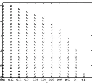
Δpi = 0.2 for i = 1,2. To show the validity of derived conditions, we compare the feasible areas in the region (0.01≤ ca ≤ 0.12 and 0.01 ≤ cb ≤ 0.26 ) for the proposed robust control design method and the SOS-based design method of [36] as shown in Fig. 5. It shows that the proposed robust

design method provides more relaxed results than the method of [36].

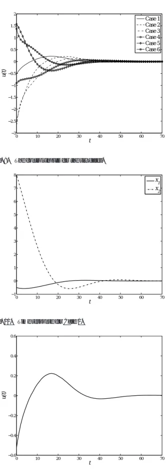
For ca = cb = 0.1, Fig. 6 shows the behavior of the nonlinear system (50) with u= 0. By solving the conditions in Theorem 1, a feasible solution for ca =cb = 0.1 can be obtained as λ= 6.806, V(x) = 1.3643x2₁+ 0.1451x2₂ F₁(x) = 1.6015x₁+ 0.3447x₂+ 0.7279 0.3447x₁+ 0.0207 T , F₂(x) = 1.6672x₁+ 0.3119x₂+ 0.7391 0.3119x₁−0.0983 T , ¯ g₁,1(x) = 0.4911x41+ 0.0476x31x2+ 0.3544x21x22 + 0.0276x3₁−0.1997x₁2x2−0.1470x1x2₂ + 0.6121x2₁−0.2999x₁x₂+ 0.2630x2₂, ¯ g₁,2(x) = 0.5928x41+ 0.1080x31x2+ 0.4294x21x22 + 0.1331x3₁−0.0122x₁2x₂−0.0341x₁x2₂ + 0.7168x2₁−0.1211x₁x₂+ 0.4064x2₂, ¯ g2,1(x) = 0.5621x4₁+ 0.1221x3₁x2+ 0.4267x2₁x2₂ + 0.1256x3₁+ 0.0282x₁2x₂−0.0193x₁x2₂ + 0.7251x2₁−0.1052x₁x₂+ 0.3879x2₂, ¯ g₂,2(x) = 0.5316x41+ 0.0840x31x2+ 0.3902x21x22 + 0.1579x3₁+ 0.1456x₁2x2+ 0.0557x1x2₂ + 0.6790x2₁−0.1412x₁x₂+ 0.3752x2₂.

Fig. 7 shows the controlled behavior for six different initial conditions. It can be seen from Fig. 7 that the design fuzzy controller stabilizes the system from all the initial conditions although the system has uncertainties.

Remark 7. Design Examples I and II show that our approach provides more relaxed results than the existing LMI approach and the existing SOS approach. In addition, as mentioned in

0.01 0.02 0.03 0.04 0.05 0.06 0.07 0.08 0.09 0.1 0.11 0.01 0.05 0.1 0.15 0.2 0.25 c a cb

Fig. 5. Feasible areas for proposed robust control design method () and the SOS-based design method of [36] (*).

−10 −8 −6 −4 −2 0 2 4 6 8 10 −10 −8 −6 −4 −2 0 2 4 6 8 10 x 1 x2

Fig. 6. Behavior of the nonlinear system (50) withu= 0.

−10 −8 −6 −4 −2 0 2 4 6 8 10 −10 −8 −6 −4 −2 0 2 4 6 8 10 x 1 x2

Fig. 7. Controlled behavior of the nonlinear system (50).

Remark 6, the LMI-based approach for the T-S fuzzy model does not guarantte the global stability of the nonlinear system.

VI. SEMI-GLOBALROBUSTSTABILIZATIONCONDITIONS

WITHCONSIDERINGINPUTCONSTRAINTS

Sections III and V gave global robust stabilization condi-tions and their design examples. It is known that the global sta-bilization is sometimes difficult to be achieved for complicated systems, e.g., unmanned aerial vehicles (UAVs), in practical. Moreover, it is usually the case that the input constraints exist in practical systems. Therefore, Section VI proposes a semi-global robust control design method with considering the input constraints. Section VII will show altitude control of a paraglider-type UAV as a design example of the semi-global robust stabilization with considering the input constraints.

Consider the operation domain

Do={x:xminβ ≤xβ≤xmaxβ , β= 1, · · ·, n} (51) and input constraints