WP 19-08
Gary Koopy
University of Strathclyde, Glasgow, UK
and
The Rimini Centre for Economic Analysis, Italy
Markus Jochmann
University of Strathclyde, Glasgow, UK
and
The Rimini Centre for Economic Analysis, Italy
Rodney W. Strachan
University of Queensland, UK
and
The Rimini Centre for Economic Analysis, Italy
“B
AYESIAN
F
ORECASTING
USING
S
TOCHASTIC
S
EARCH
V
ARIABLE
S
ELECTION
IN
A
VAR S
UBJECT
TO
B
REAKS
”
Copyright belongs to the author. Small sections of the text, not exceeding three paragraphs, can be used provided proper acknowledgement is given.
The Rimini Centre for Economic Analysis (RCEA) was established in March 2007. RCEA is a private, non-profit organization dedicated to independent research in Applied and Theoretical Economics and related fields. RCEA organizes seminars and workshops, sponsors a general interest journal The Review of Economic Analysis, and organizes a biennial conference: Small Open Economies in the Globalized World (SOEGW). Scientific work contributed by the RCEA Scholars is published in the RCEA Working Papers series.
The views expressed in this paper are those of the authors. No responsibility for them should be attributed to the Rimini Centre for Economic Analysis.
Bayesian Forecasting using Stochastic Search
Variable Selection in a VAR Subject to
Breaks
Markus Jochmann
University of Strathclyde
Gary Koop
yUniversity of Strathclyde
Rodney W. Strachan
University of Queensland
June 2008
AbstractThis paper builds a model which has two extensions over a stan-dard VAR. The …rst of these is stochastic search variable selection, which is an automatic model selection device which allows for coe¢ -cients in a possibly over-parameterized VAR to be set to zero. The second allows for an unknown number of structual breaks in the VAR parameters. We investigate the in-sample and forecasting performance of our model in an application involving a commonly-used US macro-economic data set. We …nd that, in-sample, these extensions clearly are warranted. In a recursive forecasting exercise, we …nd moderate improvements over a standard VAR, although most of these improve-ments are due to the use of stochastic search variable selection rather than the inclusion of breaks.
All authors are Fellows at the Rimini Centre for Economic Analysis.
yCorresponding author: Gary Koop, Department of Economics, University of
1
Introduction
Since the so-called Minnesota revolution associated with the work of Chris Sims and colleagues at the University of Minnesota [see Doan, Litterman and Sims (1984), Litterman (1986) and Sims (1980)], Bayesian vector autoregres-sions (VARs) have become a popular and successful forecasting tool [see, among a myriad of others, Andersson and Karlsson (2007) and Kadiyala and Karlsson (1993)]. Geweke and Whiteman (2006) provide an excellent survey of the development of Bayesian VAR forecasting.
Despite the success of VARs relative to many alternatives, two problems continue to undermine their forecast performance. These are the problems of structural breaks and over-parameterization. The purpose of this paper is to investigate whether extending a VAR to allow for structural breaks and using stochastic search variable selection will help overcome these problems. With regards to the problem of over-parameterization, VARs have so many parameters that over-…tting is a serious risk. Good in-sample model …t may not necessarily lead to good forecasting performance. Furthermore, in a typical VAR, many coe¢ cients are close to zero and/or are imprecisely estimated. This can lead to a great deal of forecast uncertainty (e.g. large predictive standard deviations). As a result, most Bayesian VARs involve informative priors (e.g. the Minnesota prior) which allow for shrinkage. In-deed a wide variety of Bayesian and non-Bayesian approaches have empha-sized the importance of shrinkage to improve forecast performance. Geweke and Whiteman (2006) provide a general discussion of this issue and empirical examples include Diebold and Pauly (1990) and Koop and Potter (2004).
In this paper, we investigate an alternative way of treating the over-parameterization problem: stochastic search variable selection (SSVS). SSVS can be thought of as a hierarchical prior where each of the parameters in the VAR is drawn from one of two Normal distributions. The …rst of these has a zero mean and a variance very near to zero (i.e. the parameter is virtually zero and the corresponding variable is e¤ectively excluded from the model). The second of these is a relatively noninformative prior (i.e. the parameter is non-zero and the corresponding variable is included in the model). Such “spike and slab” priors have become popular for model selection or model averaging in regression models [see, e.g., Ishwaran and Rao (2005)]. George, Sun and Ni (2008) develop a particular way of implementing SSVS in VAR models and Korobilis (2008) presents an application in a factor model. In this paper we use a VAR with SSVS (extended to allow for structural breaks as
described below) in a recursive forecasting exercise. Note that this approach can be thought of as a way of doing shrinkage (i.e. some coe¢ cients are shrunk virtually to zero, while others are left relatively unconstrained and estimated in a data based fashion). In our recursive forecasting exercise it also allows us to see if the set of variables which are useful predictors changes over time.
With regards to the second problem, several recent papers have high-lighted the fact that structural instability seems to be present in a wide vari-ety of macroeconomic and …nancial time series [e.g. Ang and Bekaert (2002) and Stock and Watson (1996)]. The negative consequences of ignoring this instability for inference and forecasting has been stressed by, among many others, Clements and Hendry (1998, 1999), Koop and Potter (2001, 2007) and Pesaran, Pettenuzzo and Timmerman (2006). If a structural break occurs, then pre-break data can potentially contaminate forecasts. In this paper, we adopt an approach similar to Chib (1998) to modelling the break process. This approach assumes that there is a constant probability of a break in every time period and implies that our forecasts use only data since the most recent break. Furthermore, as outlined in Koop and Potter (2007) and Pe-saran, Pettenuzzo and Timmerman (2006), such an approach allows for the possibility that a structural break might hit during the forecast period.
After building our model, which extends the VAR to allow for structural breaks and uses the SSVS hierarchical prior, we use it in a recursive fore-casting exercise using US data. In particular, we work with three variables: the unemployment rate, the interest rate and the in‡ation rate. The original data runs from 1953Q1 through 2006Q3. We compare our full model (the VAR with SSVS plus breaks) to two restricted versions: a standard VAR with SSVS and a standard VAR without SSVS. We present in-sample results which indicate that the full model outperforms both restricted variants. We then present a battery of evidence from a recursive forecasting exercise. This evidence shows that SSVS o¤ers an appreciable improvement in forecast per-formance. Evidence that the inclusion of structural breaks improves forecast performance in this data set is weaker.
2
The VAR with SSVS Prior and Structural
Breaks
The models used in this paper all begin with an unrestricted VAR which we write as:
yt+h =Xt +"t; (1)
where yt+h is an n 1 vector of observations on the dependent variables at
time t+h, aK 1vector of VAR coe¢ cients, "tare independentN(0; )
errors for t = 1; ::; T. Xt is the n K matrix containing the dependent
variables at time t through time t p + 1 (i.e. Xt contains information
available at time t) and an intercept [arranged appropriately to de…ne a VAR(p)]. The forecast horizon is h.
To this foundation, we add the SSVS prior and allow for structural breaks. In this section, we describe how this is done, with full details of our Bayesian econometric methods, including the Markov chain Monte Carlo algorithm, described in the appendix.
2.1
Stochastic Search Variable Selection
SSVS is usually motivated as a method for selecting variables in a regression model. However, it can also be interpreted as a hierarchical prior for (1). In this section, we will describe the basic ideas of SSVS as it relates to the VAR coe¢ cients, = ( 1; ::; K)0. However, we also apply SSVS to the
o¤-diagonal elements of , allowing for each of these to be shrunk virtually to zero (we do not allow for the diagonal elements of to be shrunk to zero since then it would be singular). Full details are given in the appendix.
The SSVS prior for each VAR coe¢ cient is a mixture of two Normals:
jj j 1 j N 0; 20j + jN 0; 21j ; (2)
where j is a dummy variable which equals 1 if j is drawn from the …rst
Normal and equals 0 if it is drawn from the second. The prior is hierarchical since = ( 1; ::; K)0 is treated as an unknown vector of parameters and estimated in a data-based fashion. The SSVS aspect of this prior arises by choosing the …rst prior variance, 2
0j, to be “small”(so that the coe¢ cient is
virtually zero) and the second prior variance, 2
1j, to be “large” (implying a
“small”and “large”prior variances can be chosen is discussed in, e.g., George and McCulloch (1993, 1997). Basically, the small prior variance is chosen to be small enough so that the corresponding explanatory variable is, to all intents and purposes, deleted from the model. In this paper, we use what George, Sun and Ni (2008) call a “default semi-automatic approach” which requires no subjective prior information from the researcher (see the appendix for details).1
To understand how SSVS can be used when forecasting, note that j
can be interpreted as an indicator for whether the jth VAR coe¢ cient is
in the model or not. SSVS methods allow, at each point in time in a re-cursive forecasting exercise, for the calculation of Pr j = 0jData . SSVS can either be used as a model selection device (e.g. we can choose to fore-cast using the restricted VAR which includes only the coe¢ cients for which
Pr j = 0jData > 1
2), or it can be used to do model averaging. That is,
our MCMC algorithm provides us with draws of j for j = 1; ::; K. Each
draw implies a particular restricted VAR which we can use for forecasting. By averaging over all MCMC draws we are doing Bayesian model averaging. But we stress that Pr j = 0jData can be di¤erent at di¤erent points in time in the recursive forecasting exercise and, thus, the weights attached to di¤erent models are changing over time.
2.2
Allowing For Structural Breaks
Given the …nding of widespread structural instability in many macroeconomic time series models, it is important to allow for structural breaks (in both the conditional mean and the conditional variance) of the VAR. Accordingly, we extend the VAR with the SSVS prior to allow for breaks to occur. Our approach will allow for a constant probability of a break in each time period. With such an approach, the number of breaks, M 1, is unknown (and estimated in the model). This leads to a model with structural breaks at times 1; ::; M 1 (and, thus, M regimes exist). Thus, (1) is replaced by:
1Previously, we have referred to SSVS as allowing for coe¢ cients to be “virtually zero”
or explanatory variables being “to all intents and purposes zero”since 2
0j is not precisely
zero. In the remainder of this paper, we will omit such qualifying words and phrases like “virtually” or “to all intents and purposes”.
yt+h =Xt (1)+"t; "t N(0; (1)) fort = 1; ::; 1 yt+h =Xt (2)+"t; "t N(0; (2)) for t= 1+ 1; ::; 2 . . yt+h =Xt (M)+"t; "t N(0; (M)) for t > M 1. (3)
There are many models which could be used for the break process [see, among many others, Chib (1998), Kim, Nelson and Piger (2004), Koop and Potter (2007, 2008), Maheu and Gordon (2007), Maheu and McCurdy (2007), McCulloch and Tsay (1993), Pastor and Stambaugh (2001) and Pesaran, Pettenuzzo and Timmerman (2006)]. In this paper, we adopt a speci…cation closely related to that used in Chib (1998). It assumes that there is constant probability of a structural break occurring, q, in every time period. This is a simple, but attractive choice, since (unlike many other approaches) it does not impose a …xed number of structural breaks on the model.2 Furthermore, it allows us to predict the probability that a structural break occurs during our forecast period. Thus, it helps address one of the major concerns of macroeconomic forecasters: how to forecast when structural breaks might be occurring. In practice, our method will involve (with probability 1 q) forecasting using the VAR model which holds at time (the period the forecast is being made) and (with probabilityq) forecasting assuming a break has occurred. Similar in spirit to Maheu and McCurdy (2007) and Maheu and Gordon (2007), we assume that if a break occurs then past data provides no help with forecasting and, accordingly, forecasts are made using only prior information.3
Complete details are provided in the appendix.
3
Empirical Results
In this section, we present results working with a standard set of variables. In particular, our US data set runs from 1953Q1 through 2006Q3 and contains
2Formally, our algorithm requires the choice of a maximum number of breaks (with the
actual number of breaks occuring in-sample being estimated from the data). We choose this maximum to be large enough so as not to reasonably constrain the number of breaks.
3In contrast, Koop and Potter (2007) and Pesaran, Pettenuzzo and Timmerman (2006)
develop di¤erent models where, even after a structural break occurs, past data has some predictive power.Which alternative is preferable depends on the nature of the break process in the empirical problem under study.
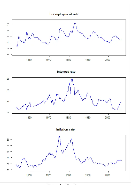
the unemployment rate (seasonally adjusted civilian unemployment rate, all workers over age 16), interest rate (yield on three month Treasury bill rate) and in‡ation rate (the annual percentage change in a chain-weighted GDP price index).4 This set of variables (possibly transformed) has been used by,
among many others, Cogley and Sargent (2005), Koop, Leon-Gonzalez and Strachan (2007) and Primiceri (2005). Figure 1 shows graphs of the three variables.
4The data were obtained from the Federal Reserve Bank of St. Louis website,
We allow for 4 lags in our VAR. This large lag length choice is motivated by our use of SSVS. That is, even if the true lag length is less than 4, the use of SSVS means that coe¢ cients on longer lags can be set to zero. We use forecast horizonsh= 1;4and8. Note thatyt+his our dependent variable and
we repeat our entire modeling exercise three times, once for each forecasting horizon. Our in-sample results are for the h= 1 case.
Note also that we are working with VARs as opposed to models which allow for cointegration. All of our variables are rates so unit root issues are likely of little importance. Ignoring unit root and cointegration issues is common practice in Bayesian macroeconomic studies. For instance, most of the work associated with Christopher Sims works with VARs [see, e.g., the citations at the beginning of the introduction or, more recently, Sims and Zha (2006)] treating cointegration as a particular parametric restriction that may or may not hold and likely to have little relevance for forecasting at short to medium horizons. Similar considerations presumably motivate recent in‡uential recent empirical macroeconomic papers such as Cogley and Sargent (2001, 2005) and Primiceri (2005) who work with VARs.
Our “default semi-automatic approach”to SSVS (see appendix) speci…es a prior for the VAR coe¢ cients. The prior for the break probability we use is given in the appendix.
We divide our discussion of empirical results into two sub-sections. In the …rst of these, we brie‡y present in-sample estimation results using the full sample. In the second, we present results for our recursive forecasting exercise.
We present empirical results for three models: the VAR with SSVS and breaks, the VAR with SSVS but no breaks and the VAR. The second model is obtained by restricting q = 0 and the third model additionally imposes
j = 1 for all parameters. The prior for any restricted model is identical
to the prior in the unrestricted model, conditional on the restriction being imposed.
3.1
In-Sample Results
Figure 2 plots the probability that a break occurs in each time period. There is evidence of two breaks, one in the mid to late 1960’s and one in the mid 1980s. That is, Figure 2 implies that the cumulative probability that a break occurs sometime in 1964-1970 is virtually one and the same holds for the 1983-1987 period. The BICs also indicate support for the model with
breaks. The BICs for the VAR, the VAR with SSVS but no breaks and the VAR with SSVS and breaks are 506.426, 388.685 and 374.904, respectively, indicating strong support for the model with breaks.5
Figure 2: Posterior Probability of a Break Occurring
Appendix B contains additional empirical results using the full sample. In particular, it contains the posterior probability of inclusion of each parameter (i.e. the probability that j = 1) as well as posterior means and standard
5In models with hierarchical priors such as ours, issues arise with how you count the
number of parameters in the penalty for complexity term in BIC (see, e.g., Carlin and Louis, 2000, pages 220-223). To avoid these complications, in models with SSVS priors we count all coe¢ cients which are included in the model with at least 16% probability.
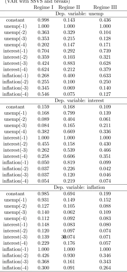
deviations for every coe¢ cient in every one of the three regimes in the VAR with SSVS and breaks. The interested reader can look through these tables in detail. Here we note two points. Firstly, it is the case that the SSVS prior is excluding (with high probability) many of the VAR coe¢ cients in each regime. This indicates that it is an e¤ective way of ensuring parsimony in the over-parameterized VAR (although, interestingly, SSVS is not deleting o¤-diagonal elements of the error covariance matrices). Secondly, in the model with breaks, although there is some evidence that some of the VAR coe¢ cients di¤er across regimes, most of the change is coming in the error covariance matrices. That is, change in the error covariance matrix is causing the breaks, not change in the VAR coe¢ cients.
3.2
Forecasting
In this section, we present results from a recursive forecasting exercise. The recursive exercise will involve using data through time to forecast +h
for h= 1;4 and 8. This will be carried out for = 0; ::; T h where 0 is 1974Q4.
Our end goal is the predictive density using information through time . We use notation where y +h is the random variable we are wishing to forecast (and y +h is the actual realization ofy +h). Thus,p y +hjX ; ::; X1 is the predictive density of interest. The properties of this density can be obtained using our MCMC algorithm. We let denote all the parameters of the VAR with breaks and m be the VAR parameters in themth regime and
(r)
m for r = 1; ::; R denote MCMC replications (subsequent to the burn-in
replications). Then, if no structural break occurs between + 1 and +h, standard MCMC theory and the structure of our model imply:
p y +hjX ; ::; X1 = 1 R R X r=1 p y +hjX ; ::; X1; (mr) (4)
asR ! 1. Note thatp y +hjX ; ::; X1; (mr) has a standard analytical form:
p y +hjX ; ::; X1; m(r) =fN(y +hjX
(r)
m;
(r)
m ); (5)
where fN denotes the normal density.
When we allow for structural breaks to occur with probabilityq, a slight extension is required. At each draw of our MCMC algorithm, we have the
VAR coe¢ cients and error covariance matrix in the last regime (i.e. using data since the last structural break) and a draw of q. With probability1 q, the predictive density is given by (5). With probabilityqa break has occurred and the predictive is based on the SSVS prior (see the Technical Appendix for details).
Once we have p y +hjX ; ::; X1 we have to choose some methods for evaluating forecast performance. We use mean squared forecast error, mean absolute forecast error, predictive likelihoods and hit rates for this purpose. The …rst two of these are based on point forecasts and are de…ned as:
M SF E= PT h = 0[y +h E(y +hjX ; ::; X1)] 2 T h 0+ 1 and M AF E = PT h = 0jy +h E(y +hjX ; ::; X1)j T h 0+ 1 :
Mean squared forecast error can be decomposed into the variance of forecast errors plus their bias squared. To aid in interpretation, we also present this bias squared (with the variance term being MSFE minus this).
Predictive likelihoods are motivated and described in many places such as Geweke and Amisano (2007). The basic predictive likelihood is the predictive density for y +h evaluated at the actual outcome y +h. We use the sum of
log predictive likelihoods for forecast evaluation:
T h
X
= 0
log p y +h =y +hjX ; ::; X1
where each term in the summation can be approximated using MCMC output in a method similar to (4).
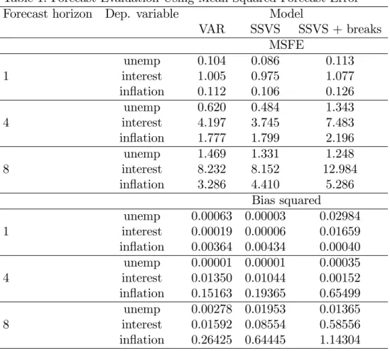
Table 1 presents MSFE and bias squared, Table 2 presents MAFE and Table 3 presents the forecast performance metric based on predictive likeli-hoods for our three models, three variables and three forecast horizons. They tell a similar story. Adding SSVS to the benchmark VAR typically improves forecast performance, but adding breaks does not. We elaborate on these points next.
Tables 1 and 2 indicate that (with the exception of in‡ation at longer horizons), the SSVS prior is helping to improve forecast performance. Rel-ative to results found in other forecasting studies, a reduction in the square
root of MSFE of 10% indicates a substantial improvement in forecast per-formance. For the unemployment rate, SSVS is leading to improvements of this magnitude (particularly at short and medium horizons). For the interest rate, there are also appreciable improvements in forecast performance. Even for the in‡ation rate (a variable which is notoriously di¢ cult to forecast), at short horizons, including SSVS does lead to some forecast improvement.
However, the inclusion of breaks does not improve forecast performance in this data set. In fact, with one exception, it leads to a deterioration of forecast performance. This sort of …nding is common in forecasting studies (see, e.g., Dacco and Satchell, 1999). Models with high dimensional parameter spaces which …t well in-sample, often do not forecast well. Even use of the SSVS prior, which is intended to help overcome the problems caused by over-parameterization, does not fully overcome this problem in this data set. The results relating to forecast bias in Table 1 shed more light on the poor forecasting performance of the model with breaks. It can be seen that all of our models are producing forecasts which are on average approximately unbiased. It is clearly the variance component that is driving the MSFE. This is consistent with the idea that the predictive density for the SSVS-with-breaks model is too dispersed. After a break occurs, our model begins estimating a new VAR using only data since the break. The advantages and disadvantages of such a strategy have been discussed in the literature. A particularly lucid exposition is provided in Pastor and Stambaugh (2001) in an empirical exercise involving the equity premium:
In standard approaches to models that admit structural breaks, estimates of current parameters rely on data only since the most recent estimated break. Discarding the earlier data reduces the risk of contaminating an estimate ... with data generated under a di¤erent [process]. That practice seems prudent, but it contends with the reality that shorter histories typically yield less precise estimates. Suppose a shift in the equity premium occurred a month ago. Discarding virtually all of the historical data on eq-uity returns would certainly remove the risk of contamination by pre-break data, but it hardly seems sensible in estimating the current equity premium. Completely discarding the pre-break data is appropriate only when the premium might have shifted to such a degree that the pre-break data are no more useful ..., than, say, pre-break rainfall data, but such a view almost surely ignores
economics [Pastor and Stambaugh, 2001, pages 1207-1208].
Our approach, by discarding all pre-break data, reduces the risk that our forecasts are contaminated by data from a di¤erent data generating process, but our resulting predictives are less precisely estimated. At least in the present application, this latter factor is clearly causing problems. Note that there do exist other Bayesian approaches which allow for pre-break data to play at least some role in post-break estimation (thus potentially leading to more precise forecasts). Examples include Pesaran, Pettenuzzo and Timmer-man (2006) and Koop and Potter (2007).
Table 1: Forecast Evaluation Using Mean Squared Forecast Error Forecast horizon Dep. variable Model
VAR SSVS SSVS + breaks MSFE unemp 0.104 0.086 0.113 1 interest 1.005 0.975 1.077 in‡ation 0.112 0.106 0.126 unemp 0.620 0.484 1.343 4 interest 4.197 3.745 7.483 in‡ation 1.777 1.799 2.196 unemp 1.469 1.331 1.248 8 interest 8.232 8.152 12.984 in‡ation 3.286 4.410 5.286 Bias squared unemp 0.00063 0.00003 0.02984 1 interest 0.00019 0.00006 0.01659 in‡ation 0.00364 0.00434 0.00040 unemp 0.00001 0.00001 0.00035 4 interest 0.01350 0.01044 0.00152 in‡ation 0.15163 0.19365 0.65499 unemp 0.00278 0.01953 0.01365 8 interest 0.01592 0.08554 0.58556 in‡ation 0.26425 0.64445 1.14304
Table 2: Forecast Evaluation Using Mean Absolute Forecast Error Forecast horizon Dep. variable Model
VAR SSVS SSVS + breaks unemp 0.210 0.200 0.255 1 interest 0.608 0.606 0.657 in‡ation 0.248 0.240 0.251 unemp 0.633 0.577 0.843 4 interest 1.509 1.446 1.945 in‡ation 0.898 0.911 1.179 unemp 0.905 0.883 0.924 8 interest 2.166 2.215 2.850 in‡ation 1.274 1.485 2.096
The poor forecast performance of the model with breaks exhibited in Ta-bles 1 and 2, could partly be due to the fact that they are based on point forecasts.6 As we saw in the preceding section, most of the evidence for
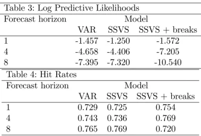
breaks seems to arise due to breaks in the conditional variance (i.e. the error covariances are changing over time), not the conditional mean (i.e. the VAR coe¢ cients are exhibiting little change over time). Loosely speaking, point forecasts largely re‡ect the conditional mean, not the conditional variance. Hence, the breaks in conditional variance are not contaminating our fore-casts from the VARs without breaks. However, the log predictive likelihoods incorporate all aspects of the predictive distribution and, hence, Table 3 in-dicates that this argument does not tell the whole story. That is, even using predictive likelihoods, we are …nding the model which allows for breaks does not forecast well.
As a …nal exercise, to see how well our predictive densities are …tting in the tails of the distribution, we calculate hit rates for a rare but important event. This event is that the unemployment and in‡ation rate both rise. A “Hit”is de…ned as occurring if the event occurs and the point forecast also lies in the region de…ned by the even. The “Hit Rate”is the proportion of Hits. Table 4 presents the Hit Rates for our various models and forecast horizons. These Hit Rates are all reasonably high, being in excess of 0.70. At very short horizons, the VAR using SSVS and breaks does have an appreciably higher hit rate, although this …nding does not occur at longer horizons.
Table 3: Log Predictive Likelihoods Forecast horizon Model
VAR SSVS SSVS + breaks 1 -1.457 -1.250 -1.572 4 -4.658 -4.406 -7.205 8 -7.395 -7.320 -10.540
Table 4: Hit Rates
Forecast horizon Model
VAR SSVS SSVS + breaks 1 0.729 0.725 0.754 4 0.743 0.736 0.769 8 0.765 0.769 0.720
4
Conclusions
In this paper, we develop a model which has two major extensions over a standard VAR. The …rst of these is SSVS and the second is breaks in all the model parameters. The motivation for the …rst is that VARs have a large number of parameters (with many of them being insigni…cant in empirical applications). This can lead to over-parameterization problems: over-…tting in-sample along with imprecise inference. The hope is that SSVS will mitigate these problems. The motivation for the second is that structural breaks are often observed to occur in macroeconomic data sets and a forecasting procedure which ignores them could be seriously misleading.
We investigate the in-sample and forecasting performance of our model in an application involving a standard trivariate VAR with three popular macroeconomic variables. Our …ndings are mixed, but are moderately en-couraging. In-sample, the VAR with SSVS and breaks clearly performs better than either a VAR with SSVS or a standard VAR. In our recursive forecasting exercise, the use of SSVS in the VAR does bring substantial improvements relative to a standard VAR. However, there is little evidence that the further addition of breaks improves forecasting performance.
References
Andersson, M. and Karlsson, S. (2007). “Bayesian forecast combination for VAR models,”forthcoming in S. Chib, W. Gri¢ ths, G. Koop and D. Ter-rell (eds.), Advances in Econometrics, Volume 23: Bayesian Econometrics,
(Elsevier: Amsterdam). Manuscript available at http://www.bus.lsu.edu/hill/aie/karlsson.pdf. Ang, A. and Bekaert, G. (2002). “Regime switches in interest rates,”
Journal of Business and Economic Statistics, 20, 163-182.
Carlin, B. and Louis, T. (2000). Bayes and Empirical Bayes Methods for
Data Analysis, second edition. (Chapman and Hall: Boca Raton).
Chib, S. (1998). “Estimation and comparison of multiple change-point models,”Journal of Econometrics, 86, 221-241.
Clements, M. and Hendry, D. (1998). Forecasting Economic Time Series. (Cambridge University Press: Cambridge).
Clements, M. and Hendry, D. (1999). Forecasting Non-stationary
Eco-nomic Time Series. (The MIT Press: Cambridge).
Cogley, T. and Sargent, T. (2001). “Evolving post-World War II in‡ation dynamics,”NBER Macroeconomic Annual, 16, 331-373.
Cogley, T. and Sargent, T. (2005). “Drifts and volatilities: Monetary policies and outcomes in the post WWII U.S,”Review of Economic Dynam-ics, 8, 262-302.
Dacco, R. and Satchell, S. (1999). “Why do regime-switching models forecast so poorly?”International Journal of Forecasting, 18, 1-16.
Diebold, F. and Pauly, P. (1990). ”The use of prior information in forecast combination,”International Journal of Forecasting, 6, 503-508.
Doan, T., Litterman, R. and Sims, C. (1984). “Forecasting and condi-tional projection using realistic prior distributions,”Econometric Reviews, 3, 1-100.
George, E. and McCulloch, R. (1993). ”Variable selection via Gibbs sam-pling,”Journal of the American Statistical Association,85, 398-409.
George, E. and McCulloch, R. (1997). ”Approaches for Bayesian variable selection,”Statistica Sinica, 7, 339-373.
George, E., Sun, D. and Ni, S. (2008). “Bayesian stochastic search for VAR model restrictions,”Journal of Econometrics, 142, 553-580.
Gerlach, R., Carter, C and Kohn, R. (2000). “E¢ cient Bayesian inference in dynamic mixture models,”Journal of the American Statistical Association, 95, 819-828.
Geweke, J. and Amisano, J. (2007). “Hierarchical Markov normal mixture models with applications to …nancial asset returns,”manuscript available at
http://www.biz.uiowa.edu/faculty/jgeweke/papers/paperA/paper.pdf. Geweke, J. and Whiteman, C. (2006). “Bayesian forecasting,” Chapter 1 in G. Elliott, C.W.J. Granger and A. Timmermann (eds.), Handbook of
Economic Forecasting. (Elsevier: Amsterdam).
Giordani, P. and Kohn, R. (2006). “E¢ cient Bayesian inference for mul-tiple change-point and mixture innovation models,”Journal of Business and Economic Statistics, forthcoming.
Ishwaran, H. and Rao, J.S. (2005). “Spike and slab variable selection: Frequentist and Bayesian strategies,”Annals of Statistics, 33, 730-773.
Kadiyala, K. and Karlsson, S. (1993). “Forecasting with generalized Bayesian vector autoregressions,”Journal of Forecasting, 12, 365-378.
Kim, C.-J., Nelson, C. and Piger, J. (2004). “The less volatile U.S. econ-omy: A Bayesian investigation of timing, breadth, and potential explana-tions,”Journal of Business and Economic Statistics, 22, 80-93.
Koop, G., Leon-Gonzalez, R. and Strachan, R. (2007). “On the evolution of monetary policy,” manuscript available at
http://personal.strath.ac.uk/gary.koop/koop_leongonzalez_strachan_kls5.pdf. Koop, G. and Potter, S. (2001). “Are apparent …ndings of nonlinearity
due to structural instability in economic time series?,”The Econometrics Journal 4, 37-55.
Koop, G. and Potter, S. (2004). “Forecasting in dynamic factor models using Bayesian model averaging,”The Econometrics Journal, 7, 550-565.
Koop, G. and Potter, S. (2007). “Estimation and forecasting in models with multiple breaks,”Review of Economic Studies, 74, 763-789.
Koop, G. and Potter, S. (2008). “Prior elicitation in multiple change-point models,”International Economic Review, forthcoming, manuscript avail-able at http://personal.strath.ac.uk/gary.koop/kp12rev.pdf
Korobilis, D. (2008). “Bayesian estimation, model selection and forecast-ing in multiple change-point models,” forthcomforecast-ing in Advances in
Econo-metrics, volume 23 (Bayesian Econometric Methods), edited by S. Chib, B.
Gri¢ ths, G. Koop and D. Terrell (Elsevier Science: Amsterdam).
Litterman, R. (1986). “Forecasting with Bayesian vector autoregressions - 5 years of experience,”Journal of Business and Economic Statistics, 4, 25-38.
Maheu, J. and Gordon, S. (2007). “Learning, forecasting and structural breaks,”Journal of Applied Econometrics, forthcoming.
Maheu, J. and McCurdy, T. (2007). “How useful are historical data for forecasting the long-run equity return distribution,”Journal of Business and
Economic Statistics, forthcoming.
McCulloch, R and Tsay, R. (1993). “Bayesian inference and prediction for mean and variance shifts in autoregressive time series,”Journal of the American Statistical Association, 88, 968-978.
Pastor, L. and Stambaugh, R. (2001). “The equity premium and struc-tural breaks,”Journal of Finance, 56, 1207-1239.
Pesaran, M.H., Pettenuzzo, D. and Timmerman, A. (2006). “Forecast-ing time series subject to multiple structural breaks,”Review of Economic Studies, 73, 1057-1084.
Primiceri. G. (2005). “Time varying structural vector autoregressions and monetary policy,”Review of Economic Studies, 72, 821-852.
Sims, C. (1980). “Macroeconomics and reality,”Econometrica, 48, 1-80. Sims, C. and Zha, T. (2006). “Were there regime switches in macroeco-nomic policy?”American Economic Review, 96, 54-81.
Stock, J. and Watson, M. (1996). “Evidence on structural instability in microeconomic time series relations,”Journal of Business and Economic Statistics, 14, 11-30.
Appendix A: Technical Details
The following are the models and associated Markov chain Monte Carlo algorithms used in the empirical section. We begin by establishing the nota-tion relating to the data. ytis ann 1vector containing data onndependent
variables and xt is a k 1 vector containing the accompanying explanatory
variables. For the VAR(p) with an intercept, xt = 1; y0t 1; ::; yt p 0 and
k = 1 +pn.
The VAR with SSVS Prior
The Likelihood Function
The VAR model can be written in matrix form as:
Y =XA+"; (A.1)
whereY is aT nmatrix withtth row given byy0
t+h,Xis aT kmatrix with tthrow given byx0t,Ais ak nmatrix of coe¢ cients and"is aT n matrix with tth row given by "0
t. The likelihood function is de…ned by assuming "t
(ann 1 vector of errors) to be i.i.d. N(0; ).
The Prior
SSVS can be interpreted as de…ning a hierarchical prior for all of the elements of A and . Each element in the hierarchy is a mixture of two normals, one with a small variance (implying the coe¢ cient is not in the model) and one with a large variance (implying the coe¢ cient is included in the model). We adopt a particular way of applying SSVS based on George, Sun and Ni (2008) and much of the material in this part of the appendix is based on their paper.
With regards to the VAR coe¢ cients, let = vec(A) with elements j
for j = 1; ::; kn:The prior for has the form:
j N(0; DD); (A.2) where is a kn 1 vector of unknown parameters with typical element
j 2 f0;1g, and D is a diagonal matrix with (j; j) th element given by dj where dj = 0j if j = 0 1j if j = 1 : (A.3)
Note that George, Sun and Ni (2008) extend (A.2) so that the prior covari-ance matrix is DRD where R is a correlation matrix which can be appro-priately chosen to allow for prior correlations between the VAR coe¢ cients.
In this paper, we assume R =I and, thus, the VAR coe¢ cients area priori
independent of one another.
Note that this prior implies a mixture of two Normals:
jj j 1 j N 0;
2
0j + jN 0;
2
1j : (A.4)
We use what George, Sun and Ni (2008) call the “default semi-automatic approach”to selecting the prior hyperparameters 0jand 1jand the reader is
referred to this paper for additional justi…cation for this approach. Basically, 0j should be selected so that j is essentially zero and 1j should be selected
so that j is empirically substantive. The default semi-automatic approach
involves 0j = c0 q d var( j) and 1j = c1 q d
var( j) where vard( j) is an
estimate of the variance of the coe¢ cient in an unrestricted VAR (e.g. the ordinary least squares quantity or an estimate based on a preliminary MCMC run of the VAR using a non-informative prior). The pre-selected constants
c0 and c1 must have c0 << c1 and we setc0 = 101 and c1 = 10.
For , the SSVS prior posits that each element has a Bernoulli form (independent of the other elements of ) and, hence, forj = 1; ::; kn, we have
Pr j = 1 =q j Pr j = 0 = 1 q j : (A.5) We set q j = 1
2 for all j. This is a natural default choice, implying each coe¢ cient is a priori equally likely to be included as excluded.
We can decompose the error covariance matrix as:
1 = 0; (A.6)
where is upper-triangular. The SSVS prior involves using a standard Gamma prior for square of each of the diagonal elements of and the SSVS mixture of normals prior for each element above the diagonal. Note that this implies that the diagonal elements of are always included in the model, ensuring a positive de…nite error covariance matrix. This form for the prior also greatly simpli…es posterior computation. Precise details are provided in the next paragraph.
Let the non-zero elements of be labelled as ijand de…ne = ( 11; ::; nn)0,
j = 1j; ::; j 1;j
0
and = ( 02; ::; 0n)0. For the diagonal elements, we as-sume prior independence with:
2
jj G aj; bj ; (A.7)
whereG aj; bj denotes the Gamma distribution with mean aj
bj and variance
aj
b2
j. We specify
aj = 2:2and bj = 0:24.
The hierarchical prior for takes the same mixture of normals form as . In particular, the SSVS prior has
jj!j N(0; FjFj); (A.8)
where !j = (!1j; ::; !j 1;j)0 is a vector of unknown parameters with typical
element !ij 2 f0;1g, and Fj =diag(f1j; ::; fj 1;j) where
fij = 0ij
if !ij = 0
1ij if !ij = 1
; (A.9)
for j = 2; ::; n and i= 1; ::; j 1.
Note that this prior implies a mixture of two Normals for each o¤-diagonal element of :
ijj!ij (1 !ij)N 0; 02ij +!ijN 0; 21ij : (A.10)
As we did with 0j and 1j (the prior hyperparameters in the SSVS for
the VAR coe¢ cients), we use a semi-automatic default approach to selecting 0ij and 1ij.That is, we set 0ij = c0
q d var ij and 1ij = c1 q d var ij
wherevar dij is an estimate of the variance of the appropriate o¤-diagonal element of from an unrestricted VAR (e.g. the ordinary least squares quantity or the posterior variance from a preliminary run of the unrestricted VAR using a noninformative prior). The pre-selected constants c0 and c1 are set (as before) to be c0 = 101 and c1 = 10.
For ! = (!02; ::; !0n)0, the SSVS prior posits that each element has a Bernoulli form (independent of the other elements of !) and, hence, we have
Pr (!ji = 1) =qji
Pr (!ji = 0) = 1 qji
: (A.11)
We make the default choice of q ji =
1
2 for all j and i.
This completes our discussion of the SSVS hierarchical prior for the VAR. Note that we also work with an unrestricted VAR. To ensure comparability
of priors across the two models, our unrestricted VAR is a limiting case of the VAR with SSVS prior. That is, our unrestricted VAR is as above except that j =!ji = 1 for all iand j.
Posterior Computation
Posterior computation can be carried out using the MCMC algorithm described in George, Sun and Ni (2008). This algorithm involves the following posterior conditional distributions. Note that, to keep the notation as simple as possible, we are suppressing the conditioning arguments, but stress that these are the full conditional posteriors necessary to describe a valid MCMC algorithm.
For the VAR coe¢ cients we have
N ; V ; (A.12) where V = ( 0) (X0X) + (DD) 1 1; =V [f( 0) (X0X)gb]; b=vec Ab and b A= (X0X) 1X0Y:
The conditional posterior for has j being independent Bernoulli
ran-dom variables: Pr j = 1 =qj Pr j = 0 = 1 qj ; (A.13) where qj = 1 1j exp 2 j 2 2 1j q j 1 1j exp 2 j 2 2 1j q j + 1 0j exp 2 j 2 2 0j 1 q j :
The conditional posterior for can be obtained by noting that the con-ditional posterior for 2jj (for j = 1; ::; n) are independent of one another
with 2 jj G aj+ T 2; bj ; (A.14) where bj = 8 < : b1+ v11 2 if j = 1 b1+ 1 2 n vjj vj0 Vj 1+ (DjDj) 1 1 vj o if j = 2; ::; n :
The preceding equation uses a notation where
V = (Y XA)0(Y XA)
has elements vij, vj = (v1j; ::; vj 1;j)0 and Vj is the upper left j j block of V.
The conditional posterior of has the conditional posteriors of j (for
j = 2; ::; n) being independent of one another with:
j N j; Vj ; (A.15) where Vj = Vj 1+ (DjDj) 1 ; j = jjVjvj:
Finally, the conditional posterior for!has!jibeing independent Bernoulli
random variables:
Pr (!ji = 1) =qji
Pr (!ji = 0) = 1 qji
; (A.16)
qji = 1 1ji exp 2 ji 2 2 1ji ! q ji 1 1ji exp 2 ji 2 2 1ji ! q ji+ 1 0ji exp 2 ji 2 2 0ji ! 1 q ji :
In summary, an MCMC algorithm for the VAR with SSVS involves se-quentially drawing from (A.12), (A.13), (A.14), (A.15) and (A.16).
The VAR with SSVS Prior and Structural Breaks at Known Points in Time
As an intermediate step to using the SSVS prior in a VAR subject to structural breaks, suppose that the breaks occur at known points in time. After each break occurs, a new regime applies and both the VAR coe¢ -cients and error covariance matrix can be completely di¤erent than before the break. Regimes will be characterized by discrete random variables, st
(for t = 1; ::; T) which takes on values f1;2; : : : ; Mg. Let Si = (s1; : : : ; si)0
and Si+1 = (s
i+1; : : : ; sT)0. Using our previously-given notation for the
de-pendent and explanatory variables, the likelihood function for our model is de…ned by assuming p(ytjxt; st=m) = p(ytjxt; m) for m = 1; : : : ; M. We
are using the generic notation m to denote the parameters in regime m.
In our VAR, m =
n
(m); (m); (m); (m); !(m)o where the parameters have the same de…nitions as above except that we are using (m) superscripts to denote parameters in each regime.
Bayesian inference, including posterior simulation, in this model is a straightforward extension of our previous results. That is, conditional on
ST, the data is broken intoM regimes. Using only the data in regimem, we
can use the algorithm described in the previous section. This can be repeated for m= 1; ::; M. Formally, we could write out this algorithm by putting(m)
superscripts on everything (i.e. on all data quantities, parameters, prior hy-perparameters) in the previous section, but for the sake of brevity we do not do so here.
The VAR with SSVS Prior and Structural Breaks at Unknown Points in Time
Our previous discussion of the model with structural breaks at known points in time suggests that a wide variety of hierarchical priors can be used for ST. An MCMC algorithm will involve taking our previous algorithm for
the VAR with SSVS prior and adding a block which draws from ST. This
is indeed the case. In this paper, we use an approach that is similar to the popular hierarchical prior for ST developed in Chib (1998). Chib’s approach
to structural break modeling has been used by many including Pastor and Stambaugh (2001) and Pesaran, Pettenuzzo and Timmerman (2006).
To implement this setup, we begin by selectingM, the maximum number of regimes. We assume that st is Markovian. That is,
Pr (st=jjst 1 =i) = 8 > > > < > > > : 1 q if j =i6=M; q if j =i+ 1; 1 if i=j =M; 0 otherwise. (A.17)
In words, the time series variable goes from regime to regime. Once it has gone through the mth regime, there is no returning to this regime. It goes
through regimes sequentially, so it is not possible to skip from regime i to regime i+ 2. Once it reaches the Mth regime it stays there. The di¤erence between the prior used in this paper and Chib’s (1998) approach is, that we choose M =T and do not assume that every regime is visited.
Equation (A.17) de…nes a hierarchical prior for the states. To complete the model, a prior for q is required. A popular choice is a Beta prior:
B( 1; 2). We select 1 = 1 and 2 = 0:01 which is a relatively noninfor-mative choice.
Bayesian inference in our model and the model of Chib (1998) is based on an MCMC algorithm. If = ( 01; : : : ; 0M)0 then the algorithm proceeds by sequentially drawing from
jY; ST; q; (A.18)
STjY; ; q (A.19)
and
pjY; ; ST: (A.20)
We have already described how to draw from (A.18). Simulation from (A.19) is done using a method developed in Chib (1996). This involves noting that:
p(STjY; ; q) = p(sTjY; ; q)p sT 1jY; ST; ; q (A.21)
p stjY; St+1; ; q p s1jY; S2; ; q :
Draws fromst can be obtained using the fact [see Chib (1996)] that p stjY; St+1; ; q /p(stjyt; ; q)p(st+1jst; q): (A.22)
Since p(st+1jst; q) is the transition probability and the integrating constant can be easily obtained (conditional on the value of st+1, st can take on only
two values), we need only to worry about p(stjyt; ; q). Chib (1996)
recom-mends the following recursive strategy. Given knowledge ofp(st 1 =mjxt; ; q) (and remembering that, in the VAR case, xt contains an intercept and lags
of the dependent variable), we can obtain:
p(st=jjyt; ; q) = Pj p(st=jjxt; ; q)p(ytjxt; j)
m=j 1p(st =mjxt; ; q)p(ytjxt; m)
; (A.23)
using the fact that
p(st=jjxt; ; q) = (1 q) p(st 1 =j 1jxt; ; q) +q p(st 1 =jjxt; ; q),
(A.24) for j = 1; ::; M.
Thus, the algorithm proceeds by calculating (A.22) for every time period using (A.23) and (A.24) beginning at t = 1 and going forward in time (the so-called forward iteration). Then the states themselves are drawn using (A.21), beginning at periodT and going backwards in time (we will refer to this as the backward iteration).
To be precise, the algorithm begins withp(s1 = 1jx1; ; q) = 1 and then uses (A.24) to calculate p(st =kjxt; ; q) for t = 2; ::; T. This allows for
everything in (A.23) to be calculated except for p(ytjxt; m). But this is
just the normal p.d.f. from the SSVS-VAR likelihood for the tth observation
(evaluated at the MCMC draw of m). Thus, (A.23) can be evaluated and
plugged into (A.22) to obtain the discrete p.d.f. p(stjY; St+1; ; q) for t = 1; ::; T:Draws from these p.d.f.s can be used in the ordering of (A.21) to draw the states (conditional on all the other parameters of the model).
Finally, derivations in McCulloch and Tsay (1993) imply that the condi-tional posterior for q is Beta:
q B 1; 2 ;
where
1 = 1+T sT
and
2 = 2+sT:
With regards to prediction, with the exception of the model with struc-tural breaks, the strategy outlined in the body of the text, using (4) and (5) applied. When breaks are present, the predictive density, conditional on the MCMC draws of the parameters, is a mixture of (5) (with probability 1 q) and the prior based quantity (with probability q). Since qis small, this prior quantity has little e¤ect but cannot be evaluated analytically due to the hi-erarchical structure of the prior. For ease of computation, we approximate it using
fN(y +hj~;~ );
where ~ and ~ are the mean vector and covariance matrix of a large number of draws from the prior predictive density.
Appendix B: Additional Empirical Results
Table B1: Probability of Inclusion of VAR coe¢ cients (VAR with SSVS, but no breaks)
Dependent variable
unemp. rate interest rate in‡ation constant 1.000 0.102 0.796 unemp(-1) 1.000 0.982 0.863 unemp(-2) 1.000 0.913 0.479 unemp(-3) 0.114 0.082 0.181 unemp(-4) 0.123 0.225 0.260 interest(-1) 0.255 1.000 0.060 interest(-2) 0.154 0.091 0.056 interest(-3) 0.772 0.762 0.047 interest(-4) 0.143 0.117 0.055 in‡ation(-1) 0.044 0.913 1.000 in‡ation(-2) 0.032 0.557 1.000 in‡ation(-3) 0.033 0.148 0.063 in‡ation(-4) 0.065 0.284 0.049 Table B2: Probability of Inclusion of O¤-Diagonal
Elements of Error Cov. (VAR with SSVS, but no breaks) unemployment rate interest rate
unemp
interest 1.000
Table B3: Probability of Inclusion of VAR coe¢ cients (VAR with SSVS and breaks)
Regime I Regime II Regime III Dep. variable: unemp constant 0.998 0.143 0.436 unemp(-1) 1.000 1.000 1.000 unemp(-2) 0.363 0.329 0.104 unemp(-3) 0.353 0.215 0.128 unemp(-4) 0.202 0.147 0.171 interest(-1) 0.704 0.292 0.739 interest(-2) 0.359 0.103 0.321 interest(-3) 0.424 0.883 0.628 interest(-4) 0.624 0.212 0.379 in‡ation(-1) 0.268 0.400 0.633 in‡ation(-2) 0.255 0.100 0.250 in‡ation(-3) 0.345 0.069 0.140 in‡ation(-4) 0.546 0.075 0.127
Dep. variable: interest constant 0.159 0.168 0.109 unemp(-1) 0.168 0.799 0.139 unemp(-2) 0.089 0.404 0.061 unemp(-3) 0.084 0.165 0.211 unemp(-4) 0.382 0.669 0.336 interest(-1) 1.000 1.000 1.000 interest(-2) 0.455 0.158 0.430 interest(-3) 0.262 0.539 0.466 interest(-4) 0.258 0.606 0.351 in‡ation(-1) 0.050 0.819 0.099 in‡ation(-2) 0.037 0.226 0.042 in‡ation(-3) 0.037 0.120 0.046 in‡ation(-4) 0.054 0.219 0.074
Dep. variable: in‡ation constant 0.985 0.694 0.199 unemp(-1) 0.931 0.149 0.152 unemp(-2) 0.127 0.105 0.088 unemp(-3) 0.140 0.062 0.109 unemp(-4) 0.112 0.092 0.083 interest(-1) 0.148 0.083 0.080 interest(-2) 0.120 0.097 0.074 interest(-3) 0.139 0.074 0.071 interest(-4) 0.229 0.176 0.057 in‡ation(-1) 1.000 1.000 1.000 in‡ation(-2) 0.426 0.930 0.346 in‡ation(-3) 0.368 0.161 0.343 30
Table B4: Probability of Inclusion of O¤-Diagonal Elements of Error Cov. (VAR with SSVS and breaks)
unemployment rate interest Regime I unemp interest 1.000 in‡ation 0.999 0.957 Regime II unemp interest 1.000 in‡ation 1.000 0.944 Regime III unemp interest 0.436 in‡ation 1.000 0.104
Table B5: Posterior Means (standard devs) of VAR coe¢ cients (VAR with SSVS and breaks)
Regime I Regime II Regime III Dep. variable: unemp
constant 1.443 (0.465) 0.018 (0.088) 0.114 (0.155) unemp(-1) 0.836 (0.180) 0.966 (0.133) 0.949 (0.089) unemp(-2) -0.095 (0.155) -0.068 (0.122) -0.004 (0.043) unemp(-3) -0.090 (0.157) -0.030 (0.069) -0.015 (0.059) unemp(-4) 0.034 (0.095) -0.005 (0.037) -0.009 (0.048) interest(-1) -0.177 (0.159) -0.015 (0.030) -0.084 (0.062) interest(-2) 0.029 (0.135) -0.001 (0.015) -0.023 (0.071) interest(-3) 0.096 (0.145) 0.088 (0.044) 0.084 (0.079) interest(-4) 0.141 (0.154) 0.011 (0.031) 0.027 (0.047) in‡ation(-1) -0.034 (0.112) 0.032 (0.040) 0.071 (0.068) in‡ation(-2) -0.063 (0.166) 0.010 (0.027) 0.028 (0.062) in‡ation(-3) -0.064 (0.240) 0.004 (0.022) 0.009 (0.041) in‡ation(-4) 0.175 (0.215) 0.002 (0.016) 0.002 (0.029)
Dep. variable: interest
constant 0.030 (0.195) 0.038 (0.254) 0.026 (0.117) unemp(-1) -0.039 (0.108) -0.902 (0.636) -0.037 (0.126) unemp(-2) 0.024 (0.093) 0.354 (0.541) 0.003 (0.072) unemp(-3) 0.015 (0.062) 0.045 (0.253) -0.099 (0.256) unemp(-4) 0.078 (0.102) 0.379 (0.334) 0.167 (0.271) interest(-1) 0.906 (0.173) 0.574 (0.175) 1.219 (0.131) interest(-2) -0.156 (0.219) 0.005 (0.052) -0.123 (0.181) interest(-3) 0.052 (0.139) 0.144 (0.165) -0.099 (0.133) interest(-4) 0.045 (0.107) 0.199 (0.195) -0.055 (0.092) in‡ation(-1) 0.004 (0.030) 0.372 (0.253) 0.017 (0.058) in‡ation(-2) 0.005 (0.045) -0.088 (0.225) 0.007 (0.052) in‡ation(-3) 0.005 (0.039) 0.014 (0.170) 0.004 (0.057) in‡ation(-4) 0.005 (0.033) -0.057 (0.144) -0.013 (0.060)
Dep. variable: in‡ation
constant 1.042 (0.346) 0.310 (0.283) 0.033 (0.087) unemp(-1) -0.167 (0.070) -0.020 (0.065) -0.023 (0.077) unemp(-2) 0.009 (0.044) 0.002 (0.055) 0.011 (0.065) unemp(-3) 0.013 (0.034) -0.000 (0.035) 0.021 (0.064) unemp(-4) 0.006 (0.023) 0.006 (0.033) 0.003 (0.028) interest(-1) -0.001 (0.022) -0.000 (0.010) 0.001 (0.011) interest(-2) 0.000 (0.023) 0.003 (0.016) -0.000 (0.014) interest(-3) 0.007 (0.038) -0.001 (0.012) -0.000 (0.014) interest(-4) -0.019 (0.052) -0.007 (0.020) 0.000 (0.009) in‡ation(-1) 1.103 (0.162) 1.521 (0.125) 1.134 (0.122) in‡ation(-2) -0.137 (0.198) -0.524 (0.190) -0.089 (0.146) in‡ation(-3) -0.076 (0.121) -0.031 (0.101) -0.058 (0.097) 32
Table B6: Posterior Means (standard devs) of Error Covariance (VAR with SSVS and breaks)
unemployment rate interest rate in‡ation Regime I unemp 2.296 (0.257) interest 1.416 2.642 (0.406) (0.290) in‡ation 0.259 -0.020 4.532 (0.433) (0.387) (0.482) Regime II unemp 3.046 (0.272) interest 2.015 1.087 (0.428) (0.111) in‡ation -0.152 -0.150 2.307 (0.438) (0.132) (0.194) Regime III unemp 5.231 (0.442) interest 2.896 2.825 (0.681) (0.231) in‡ation 0.615 -0.336 4.728 (0.746) (0.316) (0.386)
Figure B1: Boxplots of Point Forecasts for All Variables, Models and Forecast Horizons