A Taxonomy of electricity demand forecasting techniques and a selection strategy

A Taxonomy of electricity demand forecasting techniques

and a selection strategy

Paraschos Maniatis

School of Business, Department of Business Administration,

Athens University of Economics and Business,

Patision 76, GR-104 34, Athens, Greece

[email protected]

Abstract

Managerial relevance statement- This research presents a taxonomy of key electricity demand forecasting techniques that will serve as a useful reference for students, researchers, and practitioners. In addition, the research presents inputs from experts on the ratings of eight selection criteria based on World Bank policy paper for choosing a technique. Although the criteria are not adequately supported by literatures (except a few), the experts’ inputs can be useful in decision-making and future research directions.

Keywords-

1.

INTRODUCTION

In this research, a decision support model for selecting a demand forecasting method for electrical distribution industry is presented. The model is proposed based on a number of selection criteria applicable to specific demand scenarios and the objectives of forecasting. The forecasting methods are chosen from supply chain literature and applied to the electrical distribution industry with the help of a review of research studies focused on forecasting electricity demand based on consumption data and patterns. The proposed model shall be helpful to electrical engineering professionals engaged in demand planning, capacity planning, economic planning, and revenues planning in the electricity distribution industry. The Section 2 of this research presents a review of literatures on demand forecasting and the research studies its application in electricity distribution. The Section 3 presents the decision support strategy for choosing an appropriate demand forecasting method based on criteria chosen from the forecasting scenario and objectives. The strategy is presented in the form of a decision table based on inputs from 54 electrical engineers in five countries. The final section (Section 4) presents conclusions with

recommendations on using the decision support model in solving practical demand and capacity planning problems.

2.

REVIEW OF LITERATURES

2.1

The concept and techniques of demand

forecasting

Demand is a relative term to supply given that it is measured relative to supply of a product or service, from suppliers, production or from the inventory [1]. It is the key measure in determining the product/service life cycle, as presented in Figure 1 [1].

Demand forecasting is an approach to get early warning signals of customers’ requirements such that an organization can plan for adequate supplies, production, and inventory [2]. This method helps in reducing uncertainty in future by building adequate capacity to meet the projected customers’ requirements [1]. The challenge is to meet the demands without accumulating surplus capacity that may increase the overall cost of operations [2].

Demand forecasting is required for master planning in supply chains, which in turn expands into a number of intermediate plans [3]. The constraints considered are related to uncertainties in the forecasting domain (like

seasonal fluctuations) [4][5][6]. Demand forecasting helps in deciding quantitative values of the constraints such that appropriate decisions could be taken [5]. The values help in deciding a quantitative value of demands that could be met given the current constraints and the enhancement plans for expanding the boundaries such that the organization could be prepared to handle additional demands in future [5]. Demand forecasting also considers the uncertainties affecting the planning process pertaining to the constraints such that the organization can be prepared for meeting the seasonal fluctuations of demand [4][7].

Figure 1: Demand is the determiner of stages of the product/service life cycle [1]

Demand forecasting can be done using qualitative methods and quantitative techniques [8]. In this research, the focus is on quantitative techniques given that demand forecasting in electricity distribution is carried out using quantitative analysis of consumption databases (electricity load consumption in Mega Watts Hour – MWH), temperature databases, humidity databases, demographic databases, load distribution databases, and similar supporting databases [9]. The quantitative demand forecasting methods include univariate and multivariate methods [10]. Univariate methods include rule-based methods (like applying domain knowledge, different forecast horizons, bounded variables, and mapping extrapolation with trends), neural networks, and quantitative analogies (includes time series forecasting with moving averages, autoregressive progressions, Box-Jenkins method, exponential smoothing, and state-space models) [10]. Multivariate methods include causal modeling, expert systems modeling, regression analysis, segmentation (breaking the problem into independent parts), and index-based analysis (where prior knowledge of influence of variables is available) [10].

Rule-based systems help in making judgmental adjustments for improving forecasting accuracy (that is, reducing forecasting error) [11]. Judgmental adjustments help in improving system forecasting accuracy, improving

planning efficiency, reducing optimism bias, and reducing the chances of misinterpretations [11]. Using forecasting support systems and marketing intelligence data helps in extrapolation of trends, choice of right variables, and choice of upper and lower bounds [11]. Another univariate method for forecasting is the application of artificial neural networks [12]. In a feed-forward artificial neural network, the past data is divided into two sets – one for learning and another for testing [12]. The artificial neural network comprises of input nodes, hidden nodes (in hidden layers), and output nodes [12]. The output comprises the projected data series and the forecasting error in the form of mean absolute deviation, mean square error, root mean squared error, mean absolute percentage error, and sum of squared error [12]. The accuracy of the model improves with sample size [12].

Time series analysis is the most popular method for forecasting demands [13]. The most fundamental method of time series forecasting is the autoregressive integrated moving average (ARIMA; also called Box-Jenkins method) method [13]. In autoregressive modeling, a linear regression of the current value of the time series with previous values of the same series is formulated using slopes (coefficients) determined by the model parameters [13]. If M1, M2, M3, ---, Mp are the parameters of the model, the autoregressive method can be represented by the Equation (1) [14]:

Equation (1): Xt = Xmean + M1Xt-1 + M2Xt-2 + M3Xt-3 + --- + MpXt-p + At

In Equation (1), Xmean is the mean value of the series and At represents the normal distribution of random errors [14]. The moving average part of the model is based on the assumption that random shocks detected in the past are propagated in future series values [14].

Exponential smoothing is the way to assign weights to demand data before incorporating them in the moving average method [14]. Exponential smoothing induces seasonality in the demand forecasting process [15][16]. Seasonality may be additive or multiplicative depending upon how the seasonal influence appends the time series [14][16]. The additive seasonal influence is represented by Equation (2) and the multiplicative seasonal influence is represented by Equation (3) [14][15][16].

Equation (2): Xt = (A + B*t) + Ct + Ut Equation (3): Xt = (A + B*t)*Ct + Ut

Here, A is the level function, B is the linear trend function, Ct represents seasonal indices, and Ut represents a random noise function [14][15][16]. The equations (2) and (3) are point forecast models, which can be changed to state-space models by replacing “t” by “t-1” on the right hand side such that the present state of the time series is viewed as a function of the state of the time series at time “t-1” [17].

In multivariate demand forecasting models, multiple time series are analyzed using multivariate versions of ARIMA and state space models, and vector autoregressive models [18]. Multivariate forecasts are more complex because there can be higher sampling variations, more chances of

errors, model fitment issues, poor visibility into hidden relationships, and higher dependence upon background information and domain knowledge [18]. All the input variables (factors) cannot be mapped with every output variable (effect) studied [19]. Some of the relationships will be significant worth considering in the forecasting model whereas the rest will be worth discarding [19]. The significant relationships could be determined by factor-based analysis applying domain knowledge, estimating covariances, or estimating principal loading factors on the output variables [19]. The forecasting model:

M

Can be represented by Equations (4), (5), and (6) [20]. Equation (4): Y1 = L11X1 + L12X2 + L13X3 + - - - - + L1NXN + E1 Equation (5): Y2 = L21X1 + L22X2 + L23X3 + - - - - + L2NXN + E2 - - - Equation (6): YM = LM1X1 + LM2X2 + LM3X3 + - - - + LMNXN + EN

In the Equations (4), (5), and (6), LMN = factor loading, YM = variable included in the forecasting model, and XN = factors influencing the variables included in the forecasting model [20]. The factor loading significance is derived from Principal Component Analysis that helps in finding out the highest loading factors on the observed variables [20]. It can also be derived from expert systems applying past trend data and domain-level inputs [20]. The choice of which LMN variables should be included in the model depends upon their loading levels and determination of model validity [20]. In matrix notation, Equations (4), (5), and (6) can be summarized in matrix notation as shown in Equation (7).

Equation (7): Y = LX + E

L may be referred to as the structure matrix [21]. In state space notation, Equation (7) can be modified as shown in Equation (8).

Equation (8): Y = Lt-1Xt-1 + E

The term Lt-1Xt-1 may be viewed as the effect of history on the model [21]. It may be viewed as a support vector linking the observed variables in the current state with the previous state of the factors [21].

The review of demand forecasting techniques indicates that they need to be applied to appropriate scenarios depending upon the objectives of the forecasting. The criteria for selection are important for choosing the appropriate forecasting method in a forecasting project. The next section presents a review of criteria for selecting demand-forecasting techniques.

2.2

Criteria for selecting an appropriate

forecasting model for predicting demand

A demand forecasting model needs to fulfill a number of conflicting business requirements. The forecasting model

capabilities need to be chosen as per the business requirements and the preferred factors while resolving conflicting factors [22]. The key criteria for selecting an appropriate demand forecasting model are accuracy, timeliness, cost savings, interpretation ease, flexibility, data availability, user friendliness, implementation ease, judgmental inputs, reliability, developmental ease, data storage and modifications ease, theoretical reflections, and ability to compare alternative policies & environments [22][23]. The forecasting model should be based on economic fundamentals and established methods and techniques [24]. Other criteria for selecting a demand forecasting method are type of information (qualitative or quantitative), forecasting time-span (short-term, medium-term, & long-term), forecasting objectives, and goals [25]. Qualitative information causes complex decision-making challenges and diversity of opinions [25]. Hence, experts’ opinions are required to improve forecast reliability [25]. In many applications, there may be multiple predictors to be included in the forecasting model [26]. These predictors may be viewed as the factors influencing the forecasted variables with varying significances [26]. In such applications, multivariate forecasting models are created employing the techniques used for dynamic factor modeling [26]. The techniques used for dynamic factor modeling are maximum likelihood, principal component analysis, structural equation modeling, and Bayes methods [26]. In such cases, the root mean square error, the mean squared error, the mean absolute percentage error, the mean squared adjusted percentage error, mean absolute trend scaled error, mean absolute adjusted percentage error, root mean squared residual, and standardized root mean squared residual measures are helpful in choosing the most valid model comprising the factors and the forecasted variables [26][27][28][29]. Other criteria for selecting forecasting models are choice of variables, special purposes of modeling (examples are, local level modeling, local trend modeling, and seasonal modeling), and individual versus combined forecasting models [30][31][32]. The variables are chosen from a list of potential regresses applicable in the model scenario [31]. If the number of potential regressing variables is N, the number of linear models possible is 2N. In very high dimensional variables selection scenarios (where, N can be very high), the number of factors need to be reduced through factor augmentation using information selection criteria [31]. Another approach is to estimate factor loading through covariances matrix such that the factors having loading coefficients below a pre-determined level (varying from 0 to 1) can be rejected [31].

Special purposes of modeling may be needed to determine statistical underpinning for certain parameters [30]. For example, the forecaster may target estimating the weighted values of common forms of exponential smoothing [30]. Three scenarios may be considered involving the exponential smoothing parameters [30]: Equation (9): Yt = Lt-1 + αℰt (Local level modeling)

Equation (10): Yt = Lt-1 + αℰt + Bt-1 + βℰt (Local trend modeling)

Equation (11): Yt = Lt-1 + αℰt + Bt-1 + βℰt + St-m + γℰt (Seasonal modeling)

Local level modeling is a simple state space model of observations made in the sample [30]. The local trend model is a state space model of observations plus the growth/decline of observations made in the sample [30]. Seasonal level modeling is a state space model of observations plus growth/decline of observations plus seasonal components in the model [30]. The symbols α, β, and γ are smoothing parameters with the constraints 0 ≤ α ≤ 1, 0 ≤ β ≤ α, and 0 ≤ γ ≤ 1 – α [30].

2.3

Demand forecasting in power distribution

industry

As per World Bank report on energy demand models, following are the key needs of a demand forecasting model of consumer electricity [33][34]:

(a) Time horizon – short-term, medium-term, long-term (b) Accuracy level – low, medium, high

(c) Complexity – low, medium, high (d) Skills needed – low, medium, high (e) Data needed – low, medium, high

(f) Geographical coverage – low, medium, high (g) Technological coverage – low, medium, high (h) Adaptability – low, medium, high

(i) Portability – low, medium, high (from one nation to another)

(j) Cost – low, medium, high

Reference [34] added that the demand forecasting model should include impacts of system losses, load rationing, cost of energy, GDP of electricity production and population growth on electricity demand forecasting. Reference [35] added that the model should incorporate the effects of weather and temperatures on electricity load forecasting, and should have adequate explanation power such that the engineers can plan for generation and distribution lead-times. Reference [36] added a few unpredictable factors like purchase power parity, regulatory impacts, and growth of home automation appliances that are very difficult to be included in the load forecasting models.

Modeling is the aid to clear thinking and good judgment [36]. It helps in formulizing the decision problems, prepare a scope of analysis, and guide the process of decision-making [36]. In electricity demand forecasting, there are a number of factors causing uncertainties in consumption patterns [36]. On the supply side, as well, there are a number of factors affecting lead times and costs [36]. Hence, electricity demand forecasting is more complex than forecasting other forms of products and services [36].

Electricity load forecasting is primarily based on time horizon (short-term, medium-term, and long-term) [37][38][39][40]. Other needs are considered while choosing models for forecasting over a chosen time horizon [37][38][39]. The key forecasting methods used

in electricity load forecasting are the following [37][38][39][40][41][42]:

(a) Similar day approach (b) End user models

(c) State space framework with Kalman Filter (d) Multiple regression method

(e) Exponential smoothing method

(f) Multiple Regression method with Principal Component Analysis

(g) Stochastic time series

(h) Autoregressive integrated moving average model (ARIMA)

(i) Neural networks

(j) Support vector-based machine learning (k) Genetic algorithms

(l) Knowledge-based expert systems (m)Econometric models

A review of these methods is presented in the subsequent sub-sections.

2.3.1 Similar day approach

Similar day approach is a method of searching historical data over a period of one to five years for identifying days with similar load characteristics [39][44]. This exercise helps in forecasting the load of a particular day based on the load characteristics of similar days in the past [39][40][44]. The forecast data may be a linear combination or regression of load characteristics of multiple similar days in the past [39][44]. This technique can also be combined with artificial neural networks for reducing forecasting errors. This method may be rated as of low cost and moderately complex suitable for short-term load forecasts with medium accuracy level and high skills using knowledge discovery in databases, and high accuracy level and medium skills using artificial neural networks [40][43][44]. The method requires large data sets [40][44].

2.3.2 End user model

The end user model of load forecasting is based on categorization of end user consumption patterns based on a number of classifiers, like size of house, KW load allocation, electrical appliances used (lighting, cooling, heating, refrigeration, entertainment, special household machines, etc.), demographics, and such other parameters [39][44]. This method is suitable for medium and long-term electrical load forecasting [39][44]. It is highly accurate but is highly complex and expensive as it requires high levels of skills and loads of user databases [39]. This method can also be mixed with artificial neural networks and support vector machines [44].

2.3.3 State space framework with Kalman filter

The state space framework of forecasting is introduced in Section 2.1. Kalman filter is a two dimensional space of the form (24 days X 52 weeks) in which, historical demand data of a certain period is loaded [34]. This space is used to form 24 X 52 linear time-varying regression equations of the following forms [34]:

Equation (12): L (I, K) = a(K) L(I, K – 1) + b(K), K = 1, 2, 3, 4, - - - -, 24

Equation (13): L (I, K) = c(I) L(I – 1, K) + d(I), I = 1, 2, 3, 4, - - - - -, 52

The variables a(K) and b(K) are regression parameters calculated at the Kth hour.

The variable L(I, K – 1) is the weekly average load at (K – 1) hours.

The variables c(I) and d(I) are regression parameters calculated at Ith week.

The variable L(I – 1, K) is the weekly average load at (I – 1)th week.

At any discrete time instant, the load may be estimated from the Equation (14) [34]:

Equation (14): L(I, K) = α0K + α1K L(I, K – 1) + α2K L(I – 1, K) + α3K L(I – 1, K – 1)

L(I, K) = average weekly load at Ith week and Kth hour α0K = base load at Kth hour

αjK = load coefficients at Kth hour; j = 1, 2, 3

The state space model applying Kalman filter is represented by the following equations:

Equation (15): X(K + 1) = A(K)X(K) + W(K) Equation (16): Z(K) = C(K)X(K) + V(K)

X(K) and X(K + 1) denotes present and next system states, A(K) is the state transition matrix, C(K) is the output matrix, Z(K) is the measurement vector, V(K) is the measurement error, and W(K) is the system error [34]. State space modeling with Kalman’s filter is suitable for long-term forecasting with a reasonable accuracy [34]. This method is of low cost and moderate complexity requiring high skills, but requires less data (only previous year load data is sufficient). It can project hourly loads for next one year based on the hourly load data of the previous year [34].

2.3.4 Multiple regression method

The load forecast model of multiple regression method is represented by the following equation [37][38]:

Equation (17): Yt = VtAt + ℰt

Yt = Total load forecasted at the sampling time “t” Vt = a vector comprising the variables included in the forecasting model. Examples are: day (working day or a weekend), humidity, wind speed, intensity of light, and temperature.

At = a transposed vector of regression coefficients ℰt = total error in the model

This model is based on the assumption that the influencing variables chosen affect the load variation linearly and there is an internal correlation among the variables plotted on multiple time series [38][39]. This is a low cost method with moderate data requirements and moderate accuracy for short-term forecasting [37][45]. It does not require high skills because any statistical software capable of running regression reports on time series can be used [37][45]. It can help in projecting the effects of weather and temperature changes on electricity consumption patterns [37][41]. However, if high errors crop up, it is difficult to interpret their reasons [45]. The multiple regression model can be split into weather-dependent and weather-inweather-dependent parts [41]. The weather-independent part is modeled to cover the

seasonal fluctuations, and trends[41]. The weather-dependent part is influenced by cooling effects in the atmosphere (like, cloud cover) and temperatures [41]. Normally, temperature is exponentially smoothened before including in the model (the exponential smoothing technique is described in the next section) [41]. Exponential smoothing may be essential to run pre-processing commands for normalizing the loads that may have increased or decreased following an unusual trend because of unusual weather conditions [40].

2.3.5 Exponential smoothing method

The exponential smoothing model is represented by the following equation [37]:

Equation (18): Y(t) = β(t)T F(t) + ℰ(t) Y(t) = load forecasted

β(t) = Coefficient vector T = transpose operator F(t) = fitting function vector ℰ(t) = error function

The function F(t) may correspond to local level smoothing, local trend smoothing, and seasonal smoothing, as introduced in Equations (9), (10), and (11). Reference [46] presented the modified state space equations for local level, local trend, and single seasonal smoothing based on Standard Holt-Winters as presented in Equations (19), (20), and (21):

Equation (19): Local level Lt = α (Yt / St-s ) + (1 – α) (Lt-1 + Tt-1)

Equation (20): Local trend Tt = β (Lt – Lt-1) + (1 – β)Tt-1 Equation (21): Seasonality St = γ (Yt / Lt) + (1 – γ)St-s Here, α, β, and γ are smoothing parameters.

Applying the values of Lt, Tt, and St in the k-steps ahead forecasting, the Standard Holt-Winters forecasting model with single seasonal smoothing may be represented as in Equation (22) [46]:

Equation (22): Yt (k) = (Lt + kTt) St-s+k

The Standard Holt-Winters forecasting model can also be used for including double seasonality in the equation, as shown in Equations (23), (24), (25), and (26) [46]: Equation (23): Local level Lt = α (Yt / S1t-s1 S2t-s2) + (1 – α) (Lt-1 + Tt-1)

Equation (24): Local trend Tt = β (Lt – Lt-1) + (1 – β)Tt-1 Equation (25): Seasonality S1t = γ (Yt / Lt S2t-s2) + (1 – γ)S1t-s1

Equation (26): Seasonality S2t = δ (Yt / Lt S1t-s1) + (1 – δ)S2t-s2

Here, α, β, γ, and δ are smoothing parameters. The modified equation for forecasting demand with double seasonal smoothing is presented in Equation (27) [46]: Equation (27): Yt (k) = (Lt + kTt) S1t-s1+k S2t-s2+k

In the similar fashion, triple seasonal smoothing can be induced in the Standard Holt-Winters forecasting model as shown in Equation (28) [47]:

Equation (28): Yt (k) = (Lt + kTt) S1t-s1+k S2t-s2+k S3t-s3+k Reference [47] demonstrated that the demand forecasting model for electricity load can incorporate triple smoothing because of weekends, special seasons, and high temperatures. The model is suitable for including

intraday cycles, as well [47]. However, the model becomes more and more complex as multiple smoothing coefficients are included [47]. In addition, the model may not be able to predict interrelationships between two or more seasonal fluctuations [47]. The model is useful for

short-term electricity load forecasting with moderate accuracy [40][47]. However, it requires loads of data and high level of expertise for ensuring reliable forecasting outputs. The process for forecasting is presented in the Figure 2 [40].

Figure 2: Electricity load demand forecasting by combining exponential smoothing and multiple regression analysis [40] The data is normalized by eliminating unusual

event-based fluctuations (like, a major power cut due to a grid failure) and then exponential smoothing of seasonal fluctuations is applied [40]. The finalized database is transformed to prepare it for regression analysis [40]. Some operator-level adjustments may be needed to choose the input dates [40]. The finalized regressed database represents the forecasted database [40].

2.3.6 Multiple Regression method with principal

component analysis

Principal component analysis helps in reducing the number of factors in a multidimensional forecasting model in which, a large number of factors are significantly correlated with a relatively smaller number of forecast variables [48]. In electricity demand analysis, the principal component analysis method can be used to generate valid regression equations (after choosing the variables with Eigen values above unity) showing relationships between multiple seasonal factors and the load fluctuations [48]. For the Nth principal component, the regression equation can be expressed as in Equation (29) [48]:

Equation (29): PN(i) = ∑αiDi + ℰi

where, i = 1, 2, 3, 4, - - - - represents the ith day of the dataset, Di represents the day of the week, αi represents the loading value, and ℰi represents the forecasting error on the ith day of the week.

Multiple regression with Principal component analysis is a simple method with highly accurate results if the technique is applied to large sized samples [48][49]. It requires moderate software skills in tools like SPSS [50]. It helps in deriving the impact of a large number of factors on the load forecasts [49]. The forecasting expert can eliminate the factors having insignificant impacts by simply looking at the factor loading value in the output

coefficient matrix [48] [49]. Data sets from various sources can be included in the factor loading coefficients matrix irrespective of whether they are directly or indirectly related with electricity load forecasting models [49]. Reference [49]demonstrated using factors like CPI inflation and CO2 emissions, as well, in electricity load forecasting in India. For more accurate results, multiple regression with principal component analysis can be combined with artificial neural networks, as well [49].

2.3.7 Stochastic time series

Stochastic time series methods are used when the historical data sets collected from the past demand patterns comprise of some form of internal structure reflecting seasonal variations, internal trends, or autocorrelations [37][38][39]. The methods involve univariate time series employed for short-term load forecasting (typically, from one hour to seven days) using historical load demand databases [51]. A linear shift invariant filter is modeled for extrapolating input signals and producing forecasts of loads [51]. The linear shift invariant filter is represented by the formula presented in Equation (30) [51].

Equation (30): X(n) = H(z) U(n) + Wk

Here, X(n) is the input, U(n) is the output, and H(z) is the filter coefficient given by Equation (31) and Wk is a random noise factor [51].

Equation (31): H(z) = B(z) / A(z) = /

The functions a(k) and b(k) are constituents of the filter coefficient determining the signal model [51]. The modeling goal is to find out the values of a(k) and b(k) that will make X(n) closest to actual demand patterns [51].

The techniques used under stochastic time series modeling of electricity load are the following [37][38][39][52][53]:

(a) If the projected load is assumed to be a linear function of the historical loads, the autoregressive stochastic time series model may be used. Applying Burg’s autoregressive all-pole parameters, B(z) = 1, and AR model becomes as represented in Equation (32). Equation (32): X(n) = H(z) U(n) +Wk = U(n)/A(z)

+Wk = U(n) / + Wk

Autoregressive models are least accurate among all stochastic time series models but do not require significant amounts of data [53]. It is easy to understand and execute [53]. Reference [53] presented a method of improving accuracy by modifying the autoregressive model for making it multivariate. The modified model was termed as vector autoregressive model presented by Equation (33).

Equation (33): X(n) = C + H(z) U(n) + ℰk

In Equation (33), C is the K X 1 vector of constants and ℰk is the K X 1 vector of white noise. This model may be perceived to be of medium accuracy.

(b) If the projected load is not a linear function of the historical loads, the autoregressive moving average (ARMA) stochastic time series model can be adopted. It involves a state-space modeling in which, the current demand pattern plotted on a time series is matched with the demand patterns of the previous periods [(t – 1), (t – 2), (t – 3), and so on]. The periods t, (t – 1), (t – 2), (t – 3), etc. are equally spaced. The demand observations during these periods may be represented as Zt, Zt-1, Zt-2, Zt-3, and so on. B(z) is the back shift operator such that Bj X Zt = Zt-j . The autoregressive moving average model is represented by Equation (34) [52].

Equation (34): φ(B) t = (B) αt

Here, = Zt – μ, which is the deviation of observation from the mean of the observations. φ(B) is the autoregressive operator function represented by Equation (35) [52].

Equation (35): φ(B) = 1 – φ1 B – φ2 B2 – φ3 B2 – . . . – φk B2

In Equation (35), φk represents the autoregressive operator at k = 1, 2, 3, 4, - - - .

(B) is the moving average operator represented by Equation (36) [52].

Equation (36): (B) = 1 – 1B – 2 B2 – 3 B3 – . . . . – k B

p

In Equation (36), k represents the moving average operator at k = 1, 2, 3, 4, - - - .

αt is the normal distribution of residuals with zero mean and a finite variance of σα2.

Also, in ARMA model, A (z) ~ 1 / B(z) [51].

ARMA model is moderately accurate and is applicable for short-term to medium-term forecasting [54][55]. The accuracy can be improved by applying

seasonality and calendar effects. It is a complex method although data requirement is moderate (typically 2 years or more) [39][54]. The relatively more popular technique is the autoregressive integrated moving average model discussed next. (c) The autoregressive integrated moving average

(ARIMA) model is used when the forecasted load pattern has highly non-linear relationship with the historical load patterns [37][41]. This model is preferred for highly accurate electricity load forecasting when the load patterns are highly dynamic, with seasonality introduced in the model [41]. The ARIMA model with seasonality is suitable for short-term to medium-short-term modeling, although many researchers have preferred it for hourly load predictions [41]. Given its importance in electricity load forecasting, it is reviewed in a separate sub-section (2.3.8).

2.3.8 Autoregressive integrated moving average model

(ARIMA)

Power load patterns are highly dynamic with significantly stochastic series plotted over a time horizon [34][52]. Autoregressive integrated moving average model (ARIMA; also called Box-Jenkins model) offers a method for making the series static by introducing a operator as described in Equations (37), (38), and (39) [34][52].

Equation (37): = t-1 Equation (38): = ( t-1 ) = – t-1 = t-1 – t-1 + t-2 = – 2 t-1 + t-2 Equation (39): = ( t-1 ) = ( – t-1 ) = ( t-1 – t-1 + t-2 ) = ( – 2 t-1 + t-2 ) = t-1 – 2 ( t-1 + t-2 ) + t-2 + t-3 = 3 t-1 – t-2 + t-3

The equation will go on expanding in the fashion of an autoregressive integrated moving average model. The ARMA Equation (34) may be modified to ARIMA Equation (40) [34][52].

Equation (40): φ(B) t = (B) αt In Equation (40), = (1 – B)d

Further to this, seasonality can be introduced in the ARIMA equation, as in Equation (41) [34][41][52].

Equation (41): ): φ(B) t = (B)

αt

In Equation (41), is called the autoregressive seasonal operator represented by Equation (42) [34][41][52].

Equation (42): = 1 – – –

– – ……. –

In Equation (42), = autoregressive seasonal parameters at i = 1, 2, 3, 4, - - - p. The operator is the

differentiating seasonal operator defined as = (1 – Bs)D [52]. Its operation on the predicted demands yields

t = t – s [52].

The operator is the moving average seasonal operator represented by Equation (43) [34][41][52]. Equation (43): = 1 – – –

– – ……–

In Equation (43), is the moving average seasonal operator at i = 1, 2, 3, 4, - - - , q.

Seasonality can also be included with two and three cycles using the modified Holt-Winter smoothing method presented in Equation (23) through Equation (28). ARIMA becomes highly complex when seasonality is included in the model [34][41]. It requires loads of historical data that are often quite expensive to obtain [34][41]. However, ARIMA has the best accuracy and explanatory power among all stochastic time series models. It is mostly used for hourly forecasts with highly fluctuating demand data [34][41][52].

2.3.9 Artificial Neural Networks (ANNs)

Artificial Neural Network (ANN) is among the oldest explored technology for electricity load forecasting [39]. The ANN is a machine learning system comprising non-linear circuits capable of learning from a large data set

provided to them and carry out non-linear curve fitting [37][39][41]. The outputs comprise of non-linear and linear mathematical functions of the inputs provided. The inputs may be the network inputs or outputs provided by other networks. The design considerations are number formats (continuous or binary), link directions (bi-directional or uni(bi-directional), number of layers and members in them, and their connectivity. The architectures explored for electricity load forecasting using neural network are self-organizing maps, Boltzmann machine, back propagation (feed forward), radial-basis function machine, and Hopfield machine. Back propagation (feed forward) is the most popular architecture used in electricity load forecasting [39][41]. It comprises an input layer, an output layer, and several successive neuron layers in between whereby each neuron (i) accepts outputs from K input neurons and generates an output ] [41][60]. Here, A is the activation function, W is weight assigned to each input and i is the bias. It can be used for short-term, medium-term, and long-term electricity demand forecasting [60]. ANN helps in reducing empirical risks in the model [56]. ANN performs better than stochastic time series and state space forecasting, even with the K-filters and exponential smoothing applied [60][61].

Figure 4: Artificial Neural Network with fuzzy and linear/similar days preprocessors In practical industrial applications, the inputs to ANN are

facilitated by preprocessors for preparing fuzzy inputs (for seasonal inputs), linear time series inputs, or similar days inputs as shown in Figure 3 [60][61][62]. Fuzzy logic helps in deriving correlations among huge seasonal data sources (identifying first order and second order differences) by mapping the actual values to levels (like, low, medium, and high). ANNs needs experts to manage the forecasting process given its complexity and difficult adaptability [60].

2.3.10 Support vector-based machine learning

Support vector-based machine learning is a recent innovation evolved from the statistical learning theory. It is viewed as a superior technique compared with neural networks because it is focused on minimizing structural

risks instead of empirical risks [56]. The learning machine needs fewer learning patterns taken from the main data set with their complexities matching the main data set for obtaining a good generalization [57][58]. The learning algorithm selects an optimum set of rules taking a number of parameters (called weights) to form a nested structure [58]. The nested structure is formed in such a way that the hypothesis space H is divided into smaller spaces H1, H2, H3, H4, - - - - , Hn-1, and Hn such that H1⊂ H1⊂ H2⊂ H4 ⊂ - - - - ⊂ Hn-1⊂ Hn [58]. This forms a nested structure of the hypothesis space in which, each function is formed by the previous function that is relatively less complex than the encapsulating function [58]. The technique is used for creating a non-linear mapping using kernel functions into a higher dimensional space through minimizing structural

risks [39][56]. In this space, support vectors define linear decision boundaries using linear functions defined by Y = f(X) = W ψ(X) + B [56]. The function ψ(X) represents a non-linear mapping function taking from the input space “X” and the coefficients W and B are obtained through structural risk minimization [56]. The structural risk function is presented as in Equation (44) [56][57].

Equation (44): R(C) = (C / N) (Di, Yi) + 2

/ 2

In equation (44), =

The function

= = 1 / D, where

D is the distance between a support vector and an optimal canonical separating hyper-plane (OCSH) [58]. The second part of the Equation (43) is 2 / 2 = 1 / 2D2=

[ ] / 2 represents

the flatness of the model function [56][57][58].

C and ℰ are parameters prescribed for the risk function R(C) [56]. C is called the penalty parameter and having an upper bound of infinity and is the loss function that takes a value zero when the values forecasted are within the domain of ℰ (called the ℰ-tube) [56][57]. C has a trade-off between empirical risk and flatness of the model [56]. Both C and ℰ are determined by the model users. The optimal canonical separating hyper-plane (OCSH) with largest margin locates the support vectors (that is, the learning points closest to the plane) within the training data [58]. For locating the OCSH with largest margin, 2 should be minimized [58]. The optimization problem is formulated as in Equation (45) [57].

Equation (45): Minimize 2 / 2 given the conditions

In practical cases, (Xi, Yi) may not be approximated to ℰ given that there may be some errors represented by slack variables ξi and ξi

*

[57]. In such cases, the optimization problem may be written as in Equation (46) [57].

Equation (46): Minimize 2 / 2+ C

given the conditions

Using Lagrange multipliers, the support vector machine can be extended to non-linear functions [56]. Solving the optimization problem transposed into a primal Lagrangian form and applying Karush-Kuhn-Tucker conditions (steps have been skipped here), the final linear equation obtained is as in Equation (47).

Equation (47): f(X, αi, αi*) = W / + b, where,

W/ =

Here, , i = 1, 2, 3, …., l represents training patterns and the functions αi, αi* are Lagrangian multipliers. Equation (47) presents a linear relationship between the support vector W and the training patterns.

Reference [56]found that accuracy of support vector regression model outperformed regression methods and artificial neural networks method. The accuracy of the support vector regression is determined by C, ℰ, and a kernel function (called mapping function) . Kernel functions help in mapping the high-dimensional feature space with the input space [59]. Popular kernel functions are Gaussian kernel, Polynomial kernel, and linear kernel. Reference [59]found that MAPE varied from 0.8551 to 0.8501 and RMSE varied from 9.68 to 9.46 when sample size was varied from 50 to 500. Hence, support vector regression method is highly accurate even at low sample sizes. It is highly cost effective and easy to use because even small samples can produce accurate results.

2.3.11 Genetic algorithms

Genetic algorithms help in identifying an ARIMA series with exogenous variables (Xi modeled as Xa) . The resulting model is abbreviated as ARIMAX, known as the evolutionary algorithm for electricity load forecasting [37]. It is suitable for short-term load forecasting from one hour ahead to one week ahead with high accuracy [39]. The exogenous series can be determined using a genetic algorithm and investigated through the ARIMA model [39]. Genetic algorithms comprise of a genetic code structure (similar to the structures of genomes) that can provide near optimal solutions in highly stochastic systems using operators called cross-over, and mutation, [63]. The parameters to be chosen are population size, crossover probability, and mutation probability [63][64]. The algorithm is employed in ANNs with a fitness function assigned to the state vector space of input variables [63][64]. The fitness function is given by 1 / [1 + K ] that takes values between 0 and 1 [63][64][65]. Here, K is a scaling constant and ℰ(t) is the forecasting error given by / M

[63][64][65]. Here, Y(K) = actual output and is the

forecasted output, and M is the original state vector space tested in the model . The parent vector generates offsprings by either mutating or merging (crossing-over) members of the state vector space . In this way, if there are M members in the parent vector space, the genetic algorithm produces 2M members in the offspring vector space. The members with the best fitness values out of the offspring vector space are chosen to constitute Xa to be fed to the ARIMA model[65].

2.3.12 Knowledge-based expert systems

Knowledge-based expert systems are modeled based on actual field knowledge load forecasting captured from experts[37][39]. The knowledge captured is built in the

form of IF-THEN-ELSE rules in the form of a sequentially executing algorithm with decision rules. The rules reflect the changes in forced and natural factors that influence seasonal influence on the electricity load. In order to make the model accurate, the rules are localized (location-specific) and need to be updated regularly[37][39]. The expert systems incorporate fuzzy logic for converting system variables into states. They can be combined with ANNs for post-processing of the outcomes[66].

2.3.13 Econometric models

Econometric modeling is carried out by combining statistical techniques with economic theories for estimating electricity load profiles. The models are prepared using multivariate techniques comprising methods like principal component analysis, factor loading matrix, and exploratory factor analysis. Econometric modeling is highly useful in aggregating load profiles categorized as residential, industrial, and commercial comprising impacts of weather, economic variables, and known active components (like, utilities used in urban and rural belts)[39].

3.

DECISION STRATEGY FOR DEMAND

FORECASTING

IN

POWER

DISTRIBUTION

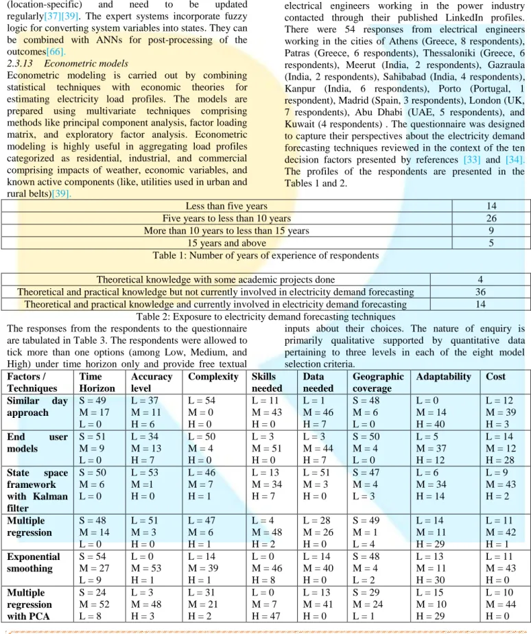
In this research, a survey questionnaire was sent to 100 electrical engineers working in the power industry contacted through their published LinkedIn profiles. There were 54 responses from electrical engineers working in the cities of Athens (Greece, 8 respondents), Patras (Greece, 6 respondents), Thessaloniki (Greece, 6 respondents), Meerut (India, 2 respondents), Gazraula (India, 2 respondents), Sahibabad (India, 4 respondents), Kanpur (India, 6 respondents), Porto (Portugal, 1 respondent), Madrid (Spain, 3 respondents), London (UK, 7 respondents), Abu Dhabi (UAE, 5 respondents), and Kuwait (4 respondents) . The questionnaire was designed to capture their perspectives about the electricity demand forecasting techniques reviewed in the context of the ten decision factors presented by references [33] and [34]. The profiles of the respondents are presented in the Tables 1 and 2.

Less than five years 14

Five years to less than 10 years 26

More than 10 years to less than 15 years 9

15 years and above 5

Table 1: Number of years of experience of respondents

Theoretical knowledge with some academic projects done 4 Theoretical and practical knowledge but not currently involved in electricity demand forecasting 36

Theoretical and practical knowledge and currently involved in electricity demand forecasting 14 Table 2: Exposure to electricity demand forecasting techniques

The responses from the respondents to the questionnaire are tabulated in Table 3. The respondents were allowed to tick more than one options (among Low, Medium, and High) under time horizon only and provide free textual

inputs about their choices. The nature of enquiry is primarily qualitative supported by quantitative data pertaining to three levels in each of the eight model selection criteria. Factors / Techniques Time Horizon Accuracy level Complexity Skills needed Data needed Geographic coverage Adaptability Cost Similar day approach S = 49 M = 17 L = 0 L = 37 M = 11 H = 6 L = 54 M = 0 H = 0 L = 11 M = 43 H = 0 L = 1 M = 46 H = 7 S = 48 M = 6 L = 0 L = 0 M = 14 H = 40 L = 12 M = 39 H = 3 End user models S = 51 M = 9 L = 0 L = 34 M = 13 H = 7 L = 50 M = 4 H = 0 L = 3 M = 51 H = 0 L = 3 M = 44 H = 7 S = 50 M = 4 L = 0 L = 5 M = 37 H = 12 L = 14 M = 12 H = 28 State space framework with Kalman filter S = 50 M = 6 L = 0 L = 53 M =1 H = 0 L = 46 M = 7 H = 1 L = 13 M = 34 H = 7 L = 51 M = 3 H = 0 S = 47 M = 4 L = 3 L = 6 M = 34 H = 14 L = 9 M = 43 H = 2 Multiple regression S = 48 M = 14 L = 0 L = 51 M = 3 H = 0 L = 47 M = 6 H = 1 L = 4 M = 48 H = 2 L = 28 M = 26 H = 0 S = 49 M = 1 L = 4 L = 14 M = 11 H = 29 L = 11 M = 42 H = 1 Exponential smoothing S = 54 M = 27 L = 9 L = 0 M = 53 H = 1 L = 14 M = 39 H = 1 L = 0 M = 46 H = 8 L = 14 M = 40 H = 0 S = 48 M = 4 L = 2 L = 13 M = 11 H = 30 L = 11 M = 43 H = 0 Multiple regression with PCA S = 24 M = 52 L = 8 L = 3 M = 48 H = 3 L = 31 M = 21 H = 2 L = 0 M = 7 H = 47 L = 13 M = 41 H = 0 S = 29 M = 24 L = 1 L = 15 M = 10 H = 29 L = 10 M = 44 H = 0

Factors / Techniques Time Horizon Accuracy level Complexity Skills needed Data needed Geographic coverage Adaptability Cost Stochastic time series except ARIMA S = 54 M = 0 L = 0 L = 54 M = 0 H = 0 L = 44 M = 10 H = 0 L = 5 M = 41 H = 8 L = 24 M = 28 H = 2 S = 1 M = 39 L = 14 L = 9 M = 12 H = 33 L = 11 M = 41 H = 2 ARIMA S = 54 M = 44 L = 0 L = 0 M = 53 H = 1 L = 31 M = 23 H = 0 L = 4 M = 41 H = 9 L = 24 M = 28 H = 2 S = 2 M = 39 L = 13 L = 8 M = 11 H = 35 L = 11 M = 40 H = 3 ANN S = 54 M = 47 L = 17 L = 0 M = 15 H = 39 L = 0 M = 13 H = 41 L = 0 M = 44 H = 10 L = 3 M = 27 H = 24 S = 44 M = 4 L = 6 L = 3 M = 15 H = 36 L = 4 M = 27 H = 23 Support Vector Regression S = 54 M = 47 L = 11 L = 0 M = 8 H = 46 L = 0 M = 5 H =49 L = 0 M = 8 H = 46 L = 54 M = 0 H = 0 S = 48 M = 6 L = 0 L = 9 M = 28 H = 17 L = 33 M = 18 H = 3 Genetic algorithms S = 54 M = 51 L = 49 L = 0 M = 18 H = 36 L = 6 M = 42 H = 6 L = 16 M = 31 H = 7 L = 4 M = 27 H = 23 S = 38 M = 14 L = 2 L = 4 M = 13 H = 37 L = 5 M = 25 H = 24 Expert systems S = 6 M = 47 L = 24 L = 13 M = 29 H = 12 L = 12 M = 5 H = 37 L = 0 M = 9 H = 45 L = 9 M = 28 H = 17 S = 53 M = 1 L = 0 L = 17 M = 16 H = 21 L = 4 M = 19 H = 31 Econometric models S = 5 M = 41 L = 49 L = 14 M = 38 H = 2 L = 34 M = 12 H = 8 L = 0 M = 1 H = 53 L = 7 M = 29 H = 18 S = 16 M = 38 L = 0 L = 18 M = 17 H = 19 L = 15 M = 21 H = 18 Table 3: Responses from the experts

The Table 3 presents ratings provided by the 54 experts to the three levels defined for each selection criterion. Excluding time horizon, skills needed, accuracy level, and data needed, the remaining four criteria are largely unaddressed by past research studies for all the techniques reviewed in this research. The World Bank policy paper is an early attempt to introduce these selection criteria (and many more, not included in this research). Comparing theoretically, the responses are in line with the research studies pertaining to time horizon, data needed and accuracy level. However, the respondents largely differ from literatures pertaining to skills needed. They have largely rated the machine learning techniques as needing high skills and the regression, exponential smoothing, state-space, and ARIMA models as needing medium skills. From the free text responses, it is found that experts find the machine learning techniques difficult to learn given that they are based on sophisticated software and model tuning is highly complex (the underlying algorithms are largely unknown). On the other hand, time-series, state space, regression, ARIMA, and exponential smoothing are easier because the experts know the underlying formulae. These techniques can be easily configured in Microsoft Excel. The free text responses also revealed that the experts rate ARIMA with exponential smoothing, Kalman filtering, or with exogenous variables (ARIMAX) as the most adopted options. As per them, the next most adopted method is the Artificial Neural Networks with preprocessed Linear and Fuzzy inputs. However, Support Vector Regression may replace this method in future as many electrical engineers are testing them in labs.

4.

CONCLUSIONS

In this research, the key techniques for electricity demand forecasting have been reviewed in the form of a taxonomy. In addition, based on an eight-factor selection criteria adopted from the World Bank policy paper, the techniques reviewed in this research are rated with the help of inputs from 54 experts. These ratings have come from experts working in electricity forecasting practice and hence may be used for selecting a technique. The criteria are not adequately supported by theories (except a few). However, the inputs from experts can be useful in making decisions about a forecasting technique and establishing future research directions. The experts rated time-horizon, accuracy level, and data needed as per the empirical theories but rated skills needed differently. From their experience, they found that the knowledge of underlying algorithms/formulations is key to developing expertise on a particular technique. The experts chose ARIMA with exponential smoothing and Kalman filtering, and ARIMAX, ANN with preprocessed linear and fuzzy inputs as the most used techniques. SVR is being explored by many experts and may replace ANN in future.

5.

REFERENCES

[1] C. Scott, H. Lundgren, & P. Thompson., "Guide to Supply Chain Management", London: Springer, 2011.

[2] M. Christopher, "Logistics and Supply Chain Management", London: Pearson, 2011.

[3] H. Stadtler, "Supply chain management and advanced planning––basics, overview and challenges", European Journal of Operational Research, 163: 575–588, Elsevier, 2005.

[4] A. Gupta, & C. D. Maranas, "Managing demand uncertainty in supply chain planning,” Computers and Chemical Engineering, 27: 1219-1227, Elsevier, 2003.

[5] R. L. Priem, & M. Swink, "A demand-side perspective on supply chain management", Journal of Supply Chain Management, 48 (2): 7-13, 2012. [6] R. H. Ballou, S. M. Gilbert, & A. Mukherjee, "New

Managerial Challenges from Supply Chain Opportunities", Industrial Marketing Management, 29: 7–18, Elsevier, 2000.

[7] M. A. Rodriguez & A. Vecchietti., "Inventory and delivery optimization under seasonal demand in the supply chain", Computers and Chemical Engineering, 34: 1705–1718, Elsevier, 2010. [8] C. Scott., H. Lundgren., & P. Thompson., "Guide to

Supply Chain Management", London: Springer, 2011.

[9] J. Campillo, F. Wallin, D. Torstensson, & I. Vassileva, "Energy demand model design for forecasting electricity consumption and simulating demand response scenarios in Sweden., In International Conference on Applied Energy ICAE 2012, July 5-8, 2012, Suzhou, China, 1-7, 2012. [10] J. S. Armstrong & K. C. Green., "Demand

Forecasting: evidence-based methods", Book Chapter: Oxford handbook in Managerial Economics", C. R. Thomas and W. F. Shughart II (Eds.), London: Oxford, 2011.

[11] R. Fildes, P. Goodwin, M. Lawrence, & K. Nikolopoulos, "Effective forecasting and judgmental adjustments: an empirical evaluation and strategies for improvement in supply-chain planning", International Journal of Forecasting, 25: 3–23, Elsevier.

[12] G. Zhang, B. E. Patuwo, & M. Y. Hu, "Forecasting with artificial neural networks: The state of the art", International Journal of Forecasting, 14: 35–62, Elsevier.

[13] J. G. De Gooijer & R. J. Hyndman, "25 years of time series forecasting", International Journal of Forecasting, 22: 443– 473, Elsevier, 2006.

[14] H. Stadtler & C. Kilger, "Supply chain management and advanced planning", London: Springer, 2005.

[15] E. Gardner, "Exponential smoothing: The state of the art-Part II, International Journal of Forecasting, 23: 637-666, Elsevier, 2007.

[16] B. Billah, M. L. King, R. D. Snyder, & A. B. Koehler, "Exponential smoothing model selection for forecasting", International Journal of Forecasting, 22: 239– 247, Elsevier.

[17] R. J. Hyndman, A. B. Koehler, R. D. Snyder, & S. Grose, "A state space framework for automatic

forecasting using exponential smoothing methods", International Journal of Forecasting, 18: 439–454, Elsevier, 2002.

[18] G. S. Pandher, "Forecasting multivariate time series with linear restrictions using constrained structural state-space models", Journal of Forecasting, 21: 281-300, Wiley, 2002.

[19] C. Chatfield, "Time-series forecasting", London: CRC Press, 2000.

[20] P. J. Brockwell & R. A. Davis, "Introduction to time-series and forecasting", second edition, NY: Springer-Verlag New York, Inc., 2002.

[21] A. De Silva, R. J. Hyndman, & R. D. Snyder, "The vector innovation structural time series framework: a simple approach to multivariate forecasting", Monash University, Australia, 2-36, 2007.

[22] J. S. Armstrong, "Selecting Forecasting Methods", Book Chapter: Principles of Forecasting: A Handbook for Researchers and Practitioners, J. Scott Armstrong (ed.): Norwell, MA: Kluwer Academic Publishers, 2001.

[23] J. T. Yokum & J. S. Armstrong, "Beyond Accuracy: Comparison of Criteria Used to Select Forecasting Methods", International Journal of Forecasting, 11 (4): 591-597, Elsevier, 1995. [24] A. Inoue & L. Kilian. “On the selection of

forecasting models”. Journal of Econometrics, 130: 273–306, Elsevier, 2006.

[25] V. Pilinkiene, "Selection of Market Demand Forecast Methods: Criteria and Application",

Engineering Economics [Online], Vol. 3 (58),

http://www.ktu.lt/lt/mokslas/zurnalai/inzeko/58/139 2-2758-2008-3-58-19.pdf?origin=publication_detail [Accessed: 28 March 2014], OALib, 2008.

[26] J. H. Stock & M. W. Watson. "Forecasting with many predictors", Book Chapter: Handbook of

Economic Forecasting, Volume 1, G. Elliott, C. W.

J. Granger, & A. Timmermann (Eds.), Elsevier, 2006.

[27] R. Poler & J. Mula, "Forecasting model selection through out-of-sample rolling horizon weighted errors", Expert Systems with Applications, 38: 14778–14785, Elsevier, 2011.

[28] B. Xu & J. Ouenniche, "Performance evaluation of competing forecasting models: A multidimensional framework based on MCDA", Expert Systems with Applications, 39: 8312–8324, Elsevier, 2012.

[29] J. W. Taylor, "Exponentially weighted information criteria for selecting among forecasting models", International Journal of Forecasting, 24: 513–524, Elsevier, 2008.

[30] B. Billah, M. L. King, R. D. Snyder, & A. B. Koehler, "Exponential smoothing model selection for forecasting", International Journal of Forecasting, 22: 239– 247, Elsevier, 2006.

[31] M. H. Pesaran, A. Pick, & A. Timmermann, "Variable selection, estimation and inference for multi-period forecasting problems", Journal of Econometrics, 164: 173–187, Elsevier.

[32] L. M. de Menezes, D. W. Bunn, & J. W. Taylor, "Review of Guidelines for the Use of Combined Forecasts", European Journal of Operational Research, 120: 190-204, Elsevier, 2000.

[33] S. C. Bhattacharya & G. R. Timilsina, "Energy Demand Models for Policy Formulation: A Comparative Study of Energy Demand Models", The World Bank Development Research Group, Environment and Energy Team, 2-151, 2009. [34] S. A. Soliman & A. M. Al-Kandai, "Electrical

Load Forecasting: Modeling and Model Construction", NY: Elsevier, 2010.

[35] C. Crowley & F. L. Joutz, "Weather Effects on Electricity Loads: Modeling and Forecasting", Department of Economics, The George Washington University, 1-48, 2005.

[36] Energy Management Forum, Electric load forecasting: Probing the issues with models, Stanford university, 1 (3), 2-55, 1979.

[37] H. K. Alfares & M. Nazeeruddin, "Electric load forecasting: literature survey and classification of methods", International Journal of Systems Science, 33 (1): 23-34, Taylor & Francis, 2002.

[38] A. K. Singh, I. S. Khatoon, M. Muazzam & D. K. Chaturvedi. "An Overview of Electricity Demand Forecasting Techniques", Network and Complex Systems, 3 (3): 38-48, 2013.

[39] E. A. Feinberg & D. Genethliou, "Electricity load forecasting", Book Chapter: Applied mathematics for restructured electrical power systems, 269-285, J. H. Chow, F. F. Wu, J. A. Momoh (Eds), London: Springer, 2005.

[40] C. Wright, C. W. Chan, & P. Laforge, "Towards Developing a Decision Support System for Electricity Load Forecast", Book Chapter: Decision Support Systems, Wright et al. (Eds), InTech, 2012. [41] H. Hahn, S. Meyer-Nieberg, S. Pickl, "Electric

load forecasting methods: Tools for decision making", European Journal of Operational Research, 199: 902–907, Elsevier, 2009.

[42] R. Weron & A. Misiorek, "Modeling and forecasting electricity loads: A comparison", In

International Conference on The European

Electricity Market EEM-04, September 20-22, 2004,

Lodz, Poland, 2004.

[43] P.Mandal, T. Senjyu, N. Urasaki, & T. Funabashi, "A neural network based several-hour-ahead electric load forecasting using similar days approach", Electrical Power and Energy Systems, 28: 367–373, Elsevier, 2006.

[44] J.Campillo, F, Wallin, D. Torstensson, & I. Vassileva, "Energy demand model designfor forecasting electricity consumption and simulating demandresponse scenarios in Sweden", In

International Conference on Applied Energy ICAE 2012, Jul 5-8, 2012, Suzhou, China, 1-7.

[45] Cullen, K. A. "Forecasting Electricity Demand using Regression and Monte Carlo Simulation Under Conditions of Insufficient Data", Published Master Thesis, West Virginia University, 1-147, 1999.

[46] J. W. Taylor. "Short-Term Electricity Demand Forecasting Using Double Seasonal Exponential Smoothing", Journal of Operational Research Society, 54: 799-805, Elsevier, 2003.

[47] J. W. Taylor. "Triple Seasonal Methods for Short-Term Electricity Demand Forecasting", European Journal of Operational Research, 204: 139-152, Elsevier, 2010.

[48] J. W. Taylor, L. M. De Menezes, & P. E. McSharry, "A comparison of univariate methods for forecasting electricity demand up to a day ahead", International Journal of Forecasting, 22: 1– 16, Elsevier, 2006.

[49] S. Saravnan, S. Kannan, & C. Thanaraj, "India's electricity demand forecast using regression analysis and artificial neural networks based on principal components", ICTACT Journal of Soft Computing, 2 (4): 365-370. 2012.

[50] H. Feng, Z. Wang, W. Ge, & Y. Wang. (2013), "Research in Residential Electricity Characteristics and Short-Term Load Forecasting", Telkomnika, 11 (12): 7021-7026.

[51] Z. Baharudin, "Autoregressive models in short-term load forecasting: a comparison of AR and ARMA", Department of Electrical & Electronics, Universiti Teknologi PETRONAS, 1-37. 2008. [52] F. A. Burney, M. Sadiq Al-Jifry, & A. B.

Esshack, "Time Series Approach to Hourly Electric Load Forecasting for the Western Province of Saudi Arabia", Journal of King Abdulaziz University (JKAU): Engineering & Science Publications, 11 (2): 69-79, 1999.

[53] C. Garcia-Ascanio & C. Mate. "Electric power demand forecasting using interval time series:A comparison between VAR and iMLP", Energy Policy, 38: 715-725, Elsevier, 2010.

[54] S. S. Pappas, L. Ekonomou, P. Karampelas, D. C. Karamousantas, S.K. Katsikas, G. E. Chatzarakis, P. D. Skafidas, "Electricity demand load forecasting of the Hellenic power system using an ARMA model", Electric Power Systems Research, 80: 256– 264, Elsevier, 2010.

[55] J. Nowicka-Zagrajek & R. Weron, "Modeling electricity loads in California: ARMA models with hyperbolic noise", Journal of Signal Processing, 82 (12): 1903-1915, Elsevier, 2002.

[56] W. Hong, "Electric load forecasting by support vector model", Applied Mathematical Modelling, 33: 2444–2454, Elsevier, 2009.

[57] D. Basak, S. Pal, & D. C. Patranabis, "Support Vector Regression", Neural Information Processing – Letters and Reviews, 11 (10): 203-224, 2007. [58] V. Kecman, "Learning and Soft Computing:

Support Vector Machines, Neural Networks, and Fuzzy Logic Models", Cambridge: The MIT Press, 2001.

[59] C. Hsu, C, Wu, S. Chen, & K. Peng, "Dynamically Optimizing Parameters in Support Vector Regression: An Application of Electricity Load Forecasting", IEEE: 30-37, 2006.

[60] J. V. Ringwood, D. Bofelli, & F. T. Murray, "Forecasting Electricity Demand on Short, Medium and Long Time Scales Using Neural Networks", Journal of Intelligent and Robotic Systems, 31: 129– 147, 2001.

[61] C. Vasar, O. Prostean, I. Filip, & I. Szeidert, "Electrical energy prediction study case based on neural networks", Department of Control System Engineering, “Politehnica” University of Timisoara, Romania, 1-8. 2004.

[62] P. Mandal, T. Senjyu, N. Urasaki, & T. Funabashi, "A neural network based several-hour-ahead electric load forecasting using similar days approach", Electrical Power and Energy Systems, 28: 367–373, 2006.

[63] K. M. El-Naggar & K. A. Al-Rumaih, "Electric Load Forecasting Using Genetic Based Algorithm, Optimal Filter Estimator and Least Error Squares Technique: Comparative Study", WASET, 6: 138-142, 2005.

[64] S. Mishra & S. K. Patra, "Short Term Load Forecasting using Neural Network trained with Genetic Algorithm & Particle Swarm Optimization", IEEE: 1-5, 2008.

[65] Y. Zhangang, C. Yanbo, K. W.E. Cheng, "Genetic Algorithm-Based RBF Neural Network Load Forecasting Model", IEEE: 1-6, 2007.

[66] K. Kim, J. Park, K. Huang, & S. Kim, "Implementation of hybrid short-term load forecasting system using artificial neural networks and fuzzy expert systems", IEEE Transactions on Power Systems, 10 (3): 1534-1539, 1995.