Studying the effect of server side constraints on the makespan of the no-wait flow shop problem with sequence dependent setup times.

1

Studying the effect of server side constraints on the makespan of the

no-wait flow shop problem with sequence dependent setup times

Hamed Samarghandi

Department of Finance and Management Science, Edwards School of Business, University of Saskatchewan, Saskatoon, Saskatchewan, Canada, S7N 5A7

[email protected]

Abstract

This paper deals with the problem of scheduling the no-wait flow shop system with sequence dependent setup times and server side constraints. No-wait constraints state that there should be no waiting time between consecutive operations of jobs. In addition, sequence dependent setup times are considered for each operation. This means that the setup time of an operation on its respective machine is dependent on the previous operation on the same machine. Moreover, the problem consists of server side constraints, i.e., not all machines have a dedicated server to prepare them for an operation. In other words, several machines share a common server. The considered performance measure is makespan. This problem is proved to be strongly NP-Hard. To deal with the problem two genetic algorithms (GA) are developed. In order to evaluate the performance of the developed frameworks, a large number of benchmark problems are selected and solved with different server limitation scenarios. Computational results confirm that both of the proposed algorithms are efficient and competitive. The developed algorithms are able to improve many of the best-known solutions of the test problems from the literature. Moreover, the effect of the server side constraints on the makespan of the test problems is explained using the computational results.

Keywords: Flow Shop Scheduling; No-wait; Sequence Dependent Setup; Makespan; Server Side Constraints; Genetic Algorithm

1.

Introduction

The no-wait flow shop problem is a special case of the classical flow shop problem, in which there should be no waiting time between successive operations of jobs. In other words, once processing is started, no interruption is permitted between operations of the same jobs. This paper also considers a

2

sequence dependent setup time for each operation. Therefore, setup time of a machine for a specific operation depends on the previous operation that is processed on that machine. Allahverdi et al. (1999) and Aldowaisan (2001) describe the importance of considering setup times in no-wait scheduling problems. In this paper, server side constraints are also considered, meaning that a number of machines are assigned a single server that is responsible for performing the setup operations on all of these machines. As a result, setup times on the machines with a common server should not overlap. Companies always look for ways to reduce waste and improve efficiency; therefore, reducing the number of servers can be used in different situations. Whether the server is a robot or a human, reducing the number of servers without sacrificing efficiency is desirable.

The considered performance measure is makespan. Following the three-field notation of the scheduling problems, the mentioned problem can be designated as F S, _Q|nowait S, _sd|C_max. King and Spachis (1980) proved that the no-wait flow shop problem with makespan performance measure

(

F no wait C

|



|

_max) can be transformed to the Asymmetric Travelling Salesperson Problem (ATSP).

Röck (1984) proved that (

F no wait C

|



|

_max) is NP-Hard. Aldowaisan (2001) transformed the no-wait flow shop problem with separable setup times and the makespan criterion

(

F no wait setup C

|



,

|

_max) to ATSP. Since F S, _Q|nowait S, _sd|C_max is a generalization of

max

|

|

F no wait C



and

F no wait setup C

|



,

|

_max, it can be inferred that F S, _Q|nowait S, _sd|C_max

is also strongly NP-Hard.

Sequence dependent setup times occur in many practical instances. Examples of such circumstances include (Samarghandi and ElMekkawy 2014a):

 Adjusting jigs and fixtures for processing different products.  Retooling multi-tool machines.

 Cleaning machines to make them ready for the next operation. Cleaning is an indispensable part of the manufacturing processes in industries such as textile, plastic, chemical, semi-conductor, pharmaceutical, and food industries.

3

Industrial applications mentioned in the literature for F S, _Q|nowait S, _sd|C_max include chemical industries (Rajendran 1994), food industries (Hall and Sriskandarajah 1996), steel production (Wismer 1972), pharmaceutical industries (Raaymakers and Hoogeveen 2000), and production of concrete products (Grabowski and Pempera 2000). Hall and Sriskandarajah (1996) provide a comprehensive review of the applications of the problem.

In this paper, a Genetic Algorithm (GA) as well as a GA with diversified local search procedure are developed to deal with F S, _Q|nowait S, _sd|C_max. Moreover, an algorithm is developed to create a feasible timetable from a given sequence. The timetabling algorithm is further coupled with the developed genetic algorithms to explore the feasible region of the problem.

Although F S, _Q|nowait S, _sd|C_max has numerous practical applications, it has received no attention in the literature. In this paper, different server limitation scenarios are considered, and computational results are compared with the results of the 2-Opt algorithm. Moreover, computational results are compared with the most competitive methods for

F no wait S

|



,

_sd

|

C

_maxfrom the literature. In fact,

F no wait S

|



,

_sd

|

C

_max can be considered as a special case of F S, _Q|nowait S, _sd|C_max.

The contribution of this paper is three-fold. First, F S, _Q|nowait S, _sd|C_max is studied in this paper for the first time; a mathematical model is developed for this problem and a number of small-instance test problems are solved to optimality. Second, the effect of adding server side constraints with different scenarios on the makespan of

F no wait S

|



,

_sd

|

C

_max is studied by applying the developed GAs to a large number of test problems. Finally, although the algorithm is developed to deal with sequence dependent setup times and server constraints, it outperforms competitive methods specifically designed for

F no wait S

|



,

_sd

|

C

_max. Computational results show that the proposed GA methods are able to find good-quality solutions for the test problems in a reasonable time. It is hoped that the presented results will be used as a benchmark by other researchers interested in solving similar scheduling problems in the future.

4

The rest of the paper is outlined as follows. Section 2 performs a literature review. Section 3 is devoted to problem description. Section 4 explains the proposed GA methods. Section 5 summarizes the computational results. Section 6 discusses the concluding remarks and future research directions.

2.

Literature Review

The first attempts to deal with the no-wait flow shop problem should be credited to Reddi and Ramamoorthy (1972), Wismer (1972), Grabowski and Syslo (1973), Bonney and Gundry (1976), King and Spachis (1980), Gangadharan and Rajendran (1993), Rajendran (1994), Glass et al. (1999), Sidney et al. (2000), and Sviridenko (2003). The two-machine no-wait flow shop problem with setup and removal times was reduced to the famous Travelling Salesperson Problem (TSP) by Gupta et al. (1997). Cheng et al. (1999) studied the problem of

F

2, 1|

S

setup c

|

_max and proposed some heuristics for the problem. Bianco et al. (1999) proposed two heuristics for the no-wait flow shop problem with release dates and sequence dependent setup times, and makespan criterion.

Aldowaisan and Allahverdi (1998) considered

F

2 |

no wait setup



,

|



C

_i and developed a heuristic algorithm for the problem. Aldowaisan (2001) performed a research on the same problem and developed a new heuristic algorithm. In addition, Aldowaisan and Allahverdi (2004) proposed six heuristics for

F no wait c

|



|

_max and considered the separable setup time in the problem of

|

|

_i

F no



wait



C

.

Sidney et al. (2000) considered the two-machine no-wait flow shop problem with anticipatory setup times and makespan and proposed a heuristic for this problem. Guirchoun et al. (2005) studied a two-stage hybrid flow shop with no-wait constraint between the two stages and proposed a heuristic to deal with the problem. Grabowski and Pempera (2005) proposed 6 meta-heuristics for

max

|

|

F no wait C



. Liu et al. (2007) proposed a particle swarm optimization with several local search

approaches. Su and Lee (2008) considered the problem of two-machine no-wait flow shop with separable setup times and single server and developed a heuristic and a branch-and-bound algorithm to

5

solve the problem. Laha and Chakraborty (2009) proposed a constructive algorithm for

max

|

|

F no wait C



.

The literature on

F no wait setup C

|



,

|

_max and

F no wait S

|



,

_sd

|

C

_max is rather limited. Problems of

F S no wait setup C

2, 1|



,

|

_max and

J

2, 1|

S no wait setup C



,

|

_maxhave been studied by Samarghandi and ElMekkawy (2011) and Samarghandi and ElMekkawy (2013a) respectively.

max

, _Q| , _sd|

F S nowait S C should be considered as a generalization of

max

2, 1|

,

|

F S no wait setup C



. Moreover, Samarghandi and ElMekkawy (2014a) studied the problem

of

F no wait S

|



,

_sd

|

C

_max. Computational results of Samarghandi and ElMekkawy (2014a) will be

used to perform several comparisons with the results of the developed algorithms in this paper. Table 1 summarizes the available literature on the subject of this paper.

6

Table 1- Literature review

Research

Problem Considered

Proposed Method

Gupta et al. (1997) Two-machine flow shop problem with

setup and removal times Reduction to TSP

Cheng et al. (1999)

F

2, 1|

S

setup C

|

_max Heuristic

Bianco et al. (1999)

F no wait release C

|



,

|

_max Heuristic Aldowaisan and Allahverdi

(1998)

F

2 |

no wait setup



,

|



C

i Heuristic

Sidney et al. (2000)

Two-machine no-wait flow shop problem with anticipatory setup times

and makespan

Heuristic Aldowaisan (2001)

F

2 |

no wait setup



,

|



C

_i Heuristic Aldowaisan and Allahverdi

(2004)

F no wait C

|



|

max Heuristic

Guirchoun et al. (2005) Two-stage hybrid flow shop with

no-wait constraint between the two stages Heuristic Grabowski and Pempera (2005)

F no wait C

|



|

_max Various meta-heuristic

Liu et al. (2007)

F no wait C

|



|

_max PSO

Su and Lee (2008)

F

2 |

no wait setup



,

|



C

_i Branch and bound

Qian et al. (2009)

F no wait C

|



|

_max Hybrid differential evolution

Pan et al. (2008a)

F no wait C

|



|

_max Hybrid PSO

Pan et al. (2008b)

F no wait C

|



|

_max Greedy algorithms

Laha and Chakraborty (2009)

F no wait C

|



|

_max Constructive heuristic Araujoa and Naganoa (2011)

F no wait S

|



,

_sd

|

C

_max Heuristic Samarghandi and ElMekkawy

(2011)

F S no wait setup C

2, 1|



,

|

max

Hybrid variable neighbourhood search Samarghandi and ElMekkawy

(2012a)

F no wait C

|



|

max Hybrid tabu search

Samarghandi and ElMekkawy

(2012b)

F no wait setup C

|



,

|

max PSO and genetic algorithm

Nagano et al. (Article in Press) F no| wait setup, |



C_i Evolutionary clustering search

Gao et al. (2012) F no| wait setup, |



C_i Hybrid harmony search

Jolai et al. (Article in Press)

No-wait flexible flow shop scheduling problem with sequence dependent setup

times

Several metaheuristics

Rabiee et al. (Article in Press)

No-wait two-machine flow shop problem with sequence dependent setup

times and probable rework

Several metaheuristics

Ying et al. (2012)

No-wait flow shop manufacturing cell scheduling problem (FMCSP) with sequence dependent family setup times

7

3.

Problem Description

3.1.

Notations and Mathematical Model

The following notation is used throughout this paper:

M

Set of machines

|

|

m



M

Number of machines

N

Set of jobs

|

|

n



N

Number of jobs i

J

Job i ij o

j

th operation of J_i ij

p Processing time of the

j

th operation of

J

_i on its respective machine i

S

Starting time of

J

_i ij o

S

Starting time of o_ij ijk

ST Setup time of o_ij if scheduled after o_kj

0

ij

ST Setup time of o_ij if J_i is the first scheduled job

ij

ST

S Starting time of the setup time of o_ij

1, 2,...,

w

SR M

w Q



 A subset of

M

which includes the machines with one assigned server

|

SR

_w

|

Number of members of

SR

_w

l



Sequence l

max

C

Makespan of



_l

Brackets are used to indicate consecutive jobs, i.e., S_{[ ]i} refers to the starting time of the job planned to be operated after ith job in a given sequence. Moreover, suppose that SR ww; 1, 2,...,Q

is a subset of

M

and presents the set of machines for which one server is assigned to perform the setups. If

Q

servers exist in a particular instance of the problem (

w



1,2,...,

Q

), then

;1

w e

SR



SR





  

w e

Q

. In other words, it is assumed that each machine is assigned to only one server. Based on the above notations, a mathematical model for F S, _Q|nowait S, _sd|C_max is as follows:

max

Min C

(1)

max oim im; 1, 2,...,

8 [ ]i j ij [ ] ; 1,2,..., 1 1,2,..., o o ij i ji S S p ST i n j m

(3)

[ ] ; 1, 2,..., 1, 2,..., 1 i j ij o o ij S S  p i n j m

(4)

[ ]i j [ ]i k [ ] ; 1,2,..., 1 , ; 1,2,..., ST ST i ki w S S ST i n j kSR jk w Q

(5)

1j 1k 1 0; , ; 1,2,..., ST ST k w S S ST j kSR jk w Q

(6)

0; 1,2,..., 1,2,..., ij o S  i n j m

(7)

0; 1, 2,..., 1, 2,..., ij ST S  i n j m

(8)

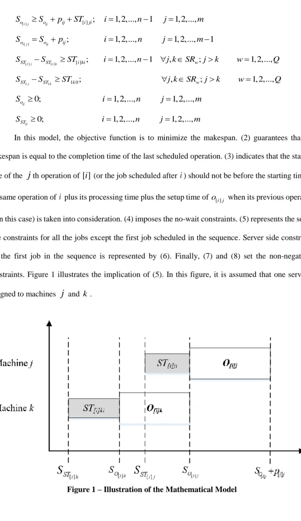
In this model, the objective function is to minimize the makespan. (2) guarantees that the makespan is equal to the completion time of the last scheduled operation. (3) indicates that the starting time of the

j

th operation of

[ ]

i

(or the job scheduled after

i

) should not be before the starting time of the same operation of

i

plus its processing time plus the setup time of o_{[ ]i j} when its previous operation (

i

in this case) is taken into consideration. (4) imposes the no-wait constraints. (5) represents the server side constraints for all the jobs except the first job scheduled in the sequence. Server side constraints for the first job in the sequence is represented by (6). Finally, (7) and (8) set the non-negativity constraints. Figure 1 illustrates the implication of (5). In this figure, it is assumed that one server is assigned to machines

j

and k.

9 Based on figure 1, one can verify that:

[ ]i j [ ]i k [ ]

ST ST i ki

S S ST

(9)

If (9) is violated, then setup times of o_{[ ]i k} and o_{[ ]i j} overlap, which is a violation of server constraints. According to (4), once the starting time of oi1 is obtained by the model, it is possible to

calculate the starting time of o_ij;j2,3,...,m. In other words, it is possible to reduce the problem to finding the best time to start o ii1; 1, 2,...,n without violating server side constraints. Consequently,

max

, _Q| , _sd |

F S nowait S C can be reduced to the Asymmetric Travelling Salesperson Problem (ATSP).

3.2.

Calculating the Makespan

An algorithm is developed here in order to calculate the objective function of

max

, _Q| , _sd |

F S nowait S C by generating a feasible timetable from a given sequence of jobs. This algorithm is called Makespan Calculation Algorithm with Server constraints or MCAS.

MCAS utilizes a pointer (

e

) and a dereference operator, denoted as

h e

( )

. A pointer refers to the place of an element in a set. For instance, if

SR

_w



{3,6,9,10}

, then e2 points to the element that is located in the second place in

SR

_w. The dereference operator shows the element that the pointer has referred to. Therefore, if e2, then

h e

( )



6

. MCAS calculates the makespan of a given permutation



_l from F S, Q|nowait S, sd|C_max.

To schedule the first job of



l:

1. Set w1.

2. Sort the indices of

SR

_w in the ascending order; suppose that |SRw|b. Define

e

as

the pointer of

SR

_w. Set e1. Set

1, ( )h e 0

ST

S  .

10 4. Set

1, ( )h e 1,( (h e1)) 1, ( ),0

ST ST h e

S S _ ST .

5. If eb, go back to step 3. If eb and

w Q



, set w w 1 and go to step 2. If eb and

w



Q

, proceed to step 6.

6. Set 11 1,1 1,1,0 o ST

S



S



ST

. 7. For k1 to m1, 1[ ]k max{ 1,[ ]k 1[ ]0, 1k 1 } O ST k O k S  S ST S p . If 1,[ ]k 1[ ]0 1k 1 ST k O k

S



ST



S



p

, set 1,[ ]k 1[ ]0

(

1k 1

)

ST k O k

d



S



ST



S



p

, and for

1,2,...,

1

z



k



, set 1z 1z O O S S d. To schedule the remaining jobs of



_l: 8. Set

i



1;

j



1

.

9. Set w1.

10. Sort the indices of

SR

_w in the ascending order; suppose that |SRw|b. Define

e

as

the pointer of

SR

_w. Set e1. Set

[ ], ( )i h e i h e, ( ) , ( ) ST o i h e S S p . 11. Set e e 1. 12. Set [ ], ( )i h e max{ [ ],( (i h e1)) [ ], ( 1),, i h e, ( ) , ( )} ST ST i h e i O i h e S  S _ ST _ S p .

13. If eb, go back to step 11. If eb and

w Q



, set w w 1 and go to step 10. If eb and

w



Q

, proceed to step 14.

14. Set [ ] [ ]i j STi ji [ ] o i ji

S



S



ST

. 15.

j

 

j

1

. 16. [ ]i j max{ [ ]i j [ ] , [ ],(i j1) [ ],( 1)} O ST i ji O i j S  S ST S _  p  . If SST_{[ ]}i j ST[ ]i ji SO_{[ ],(}i j₁₎p[ ],(i j1), set [ ]i j [ ]

(

[ ],(i j1) [ ],( 1)

)

ST i ji O i j

d



S



ST



S

_



p

_ , and for z1,2,...,j1, set

[ ]i z [ ]i z

O O

S



S



d

.

11 18. If in, stop. _max

nm o nm

C S p . Otherwise, set i i 1 and j1. Go back to step 9.

MCAS starts with a sequence of jobs (



l) or equivalently, a permutation. MCAS first schedules the sequence dependent setup times of the first job in



l based on the defined server side constraints (steps 1 to 5). Then the no-wait constraints are imposed, while modifying the starting time of the rest of the operations of that job if necessary (steps 6 and 7). When scheduling the first job of



l is completed, using the same method, MCAS first schedules the sequence dependent setup times of the next job and imposes the server constraints (steps 8 to 13). Steps 14 to 16 schedule the operations and impose the no-wait constraints. Finally, step 17 calculates the makespan and then the algorithm is completed. Computational complexity of this algorithm is O mn( ).

3.3.

Illustrative Example

Table 2 presents the data for a typical instance of F S, _Q|nowait S, _sd|C_max. For this example, all setup times are assumed to be equal to 1, except ST_2,1,13 and ST_2,2,12. Suppose that

1

{1,2}

SR



and

SR

₂



{3}

.



(1,2,3) is considered as the desired sequence and MCAS will be used to develop a timetable.

Table 2 – A Typical F S, _Q|nowait S, _sd|C_max Instance i

J p_ij

1 1 2 1

2 1 1 3

The first 5 steps of MCAS schedule the setup times of the first job in



according to the server constraints. According to step 2, MCAS sets

1,1 0

ST

S  . Since

SR

₁



{1,2}

, in step 4 MCAS sets

1,2 1,1 1,1,0 0 1 1

ST ST

S S ST    . Moreover, since

SR

₂



{3}

, which means machine 3 has its dedicated

server, MCAS sets

1,3 0

ST

12

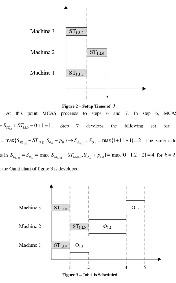
Figure 2 – Setup Times of J₁

At this point MCAS proceeds to steps 6 and 7. In step 6, MCAS sets

11 1,1 1,1,0

0 1 1

o ST

S



S



ST

  

. Step 7 develops the following set for k1:

1[ ]k

max{

1,[ ]k 1[ ]0

,

1k 1

}

1,[1] 1,2

max{1 1,1 1} 2

O ST k O k O O

S



S



ST

S



p



S



S





 

. The same calculation

results in

1,[ 2 ] 1,3

max{

1,[ 2 ] 1,[2],0

,

1,2 1,2

}

max{0 1,2 2}

4

O O ST O

S



S



S



ST

S



p









for k2. Thus,

so far the Gantt chart of figure 3 is developed.

Figure 3 – Job 1 is Scheduled

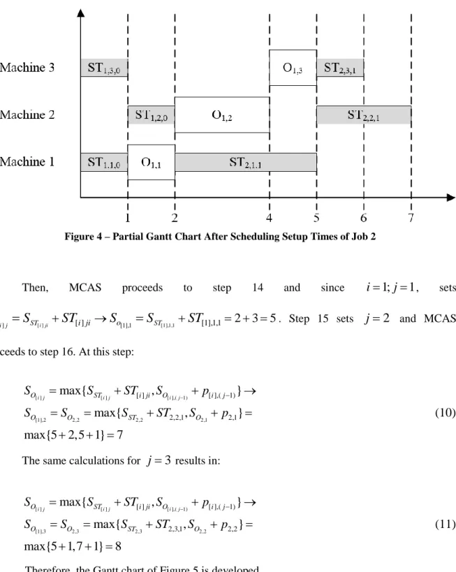
Steps 8 to 13 schedule the setup times of the second job in sequence



the same way that setup times of job 1 are scheduled. A partial Gantt chart after scheduling the setup times of job 2 is presented

13

in figure 4. Since there is one server assigned to machines 1 and 2, their setup times should not overlap. However, machine 3 has its own dedicated server and therefore its setup times can overlap with setup times of machines 1 and 2.

Figure 4 – Partial Gantt Chart After Scheduling Setup Times of Job 2

Then, MCAS proceeds to step 14 and since

i



1;

j



1

, sets

[ ] [1],1,1

[ ]i j STi ji [ ] [1],1 ST [1],1,1 2 3 5

o i ji o

S



S



ST



S



S



ST

   . Step 15 sets

j



2

and MCAS proceeds to step 16. At this step:

[ ] [ ] [ ],( 1) [1],2 2,2 2,2 2,1 [ ] [ ],( 1) 2,2,1 2,1

max{

,

}

max{

,

}

max{5 2,5 1}

7

i j i j i j O ST i ji O i j O O ST O

S

S

ST

S

p

S

S

S

ST

S

p

 





















 

(10)

The same calculations for

j



3

results in:

[ ] [ ] [ ],( 1) [1],3 2,3 2,3 2,2 [ ] [ ],( 1) 2,3,1 2,2

max{

,

}

max{

,

}

max{5 1,7 1} 8

i j i j i j O ST i ji O i j O O ST O

S

S

ST

S

p

S

S

S

ST

S

p

 





















 

(11)

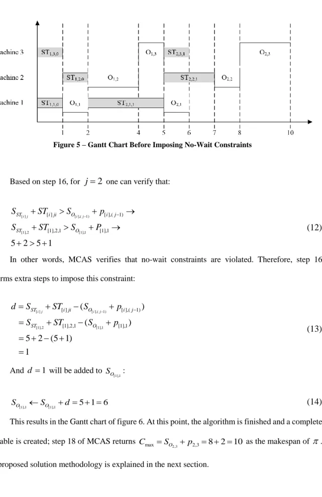
14

Figure 5 – Gantt Chart Before Imposing No-Wait Constraints

Based on step 16, for

j



2

one can verify that:

[ ] [ ],( 1) [1],2 [1],1 [ ] [ ],( 1) [1],2,1 [1],1

5 2

5 1

i j i j ST i ji O i j ST O

S

ST

S

p

S

ST

S

P

 

















  

(12)

In other words, MCAS verifies that no-wait constraints are violated. Therefore, step 16 performs extra steps to impose this constraint:

[ ] [ ],( 1) [1],2 [1],1 [ ] [ ],( 1) [1],2,1 [1],1

(

)

(

)

5 2 (5 1)

1

i j i j ST i ji O i j ST O

d

S

ST

S

p

S

ST

S

p

 

















   



(13)

And d 1 will be added to [1],1 O S : [1],1 [1],1 5 1 6 O O S S    d

(14)

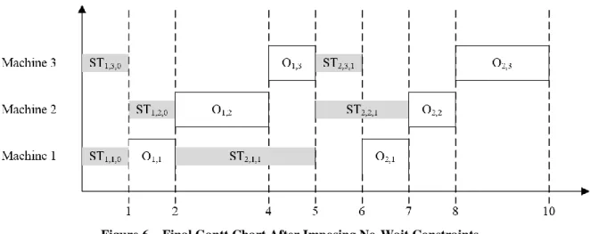
This results in the Gantt chart of figure 6. At this point, the algorithm is finished and a complete timetable is created; step 18 of MCAS returns

2,3

max O 2,3 8 2 10

C S  p    as the makespan of



.

15

Figure 6 – Final Gantt Chart After Imposing No-Wait Constraints

4.

The Proposed Genetic Algorithm

Genetic Algorithm (GA) is the main search technique in this paper. GAs are a particular class of evolutionary algorithms (EA) that use techniques inspired by evolutionary biology such as inheritance, mutation, selection, and crossover. GA uses chromosomes to code the feasible solutions of the problem. Feasible solutions of F S, _Q|nowait S, _sd|C_max are sequences of jobs, denoted by



in section 3. GA is a popular search technique with several successful implementations for the continuous and discrete optimization problems in the literature (Samarghandi and Eshghi 2009, Samarghandi et al. 2010, Samarghandi and Jahantigh 2011, Samarghandi and ElMekkawy 2013b, Samarghandi and ElMekkawy 2014b).

4.1.

Chromosome Structure and GA Operations

Chromosome structure (genotype) is one of the most important aspects of the genetic algorithm. In the proposed GA, each permutation or sequence of jobs (



) is a chromosome. MCAS generates complete and feasible timetables for F S, _Q|nowait S, _sd|C_max once a sequence of jobs is given. This approach defines the extraction of solutions from chromosomes (phenotype). It is worthwhile to mention that the proposed GA uses the operations defined by Shadrokh and Kianfar (2007).

The proposed GA generates Pop random permutations for the first generation. Then, MCAS calculates the makespan of each of these permutations. Calculated makespans will be used as the fitness label of the permutations. Pop is an even number and a parameter of the algorithm, which remains unchanged during all of the iterations of the algorithm. New generations are made from the existing generation, using four operations: crossover, mutation, immigration, and local search.

In the crossover operation, the existing generation is randomly partitioned into

2

Pop

pairs of parents, and the crossover operation is performed on each pair with probability

P

_c. If a pair is not

16

selected for crossover, each individual in this pair is considered for the mutation operation with probability

P

_m and then for local search with probability P_l.

The crossover operation on a pair of parents, P1 and

P

2, produces two children, C1 and

C

2.

Let f I( ) be the makespan of schedule

I

. If

r f P

_i

.( ( )

_i



f C

( ))

_i



f P

( )

_i then C_i will be selected for local search with probability Pl and then goes to a new generation and Pi dies out (i1, 2).

r

i is a random number generated from the interval [0,1] for each

i

. Otherwise C_i dies out and P_i is considered for mutation with probability

P

_m and then for local search with probability Pl. It should be noted that

r f P

_i

.( ( )

_i



f C

( ))

_i



f P

( )

_i determines how much advancement in the quality of genes should be expected in consecutive generations. However, since

r

_i is a random number, the amount of gene progress differs in each iteration. Afterwards, the immigration operation is also performed before finalizing the cycle of producing a new generation. Immigration operation feeds the gene pool with randomly generated genes, helps maintain the gene diversity, and helps prevent immature convergence. For the immigration operation, a chromosome will be randomly generated and is called NEW . An individual

I

is selected randomly from the current population. Let the probability of leaving

I

be

( ) ( , ) ( ) ( ) Leave f I P I NEW f I f NEW 

 . A random number is generated from the interval [0,1]. If this

random number is less than

P

_Leave

( ,

I NEW

)

, NEW replaces

I

; otherwise NEW is discarded. The immigration operation is able to bring new and desirable characteristics to the next gene pools. The chromosome with the best makespan value in the final generation is the result given by the algorithm. Pop,

P

_s,

P

_m, and Pl are adjustable parameters of the algorithm. The number of iterations of the proposed GA is another parameter of the algorithm and is denoted as

Iter

.

4.2.

Crossover

The proposed GA uses a one-point crossover. Suppose that P₁(J J₁1, 1₂,...,J_n1) and

2 2 2

2 ( 1, 2,..., n)

P  J J J are the two individuals that are selected for crossover. The one-point crossover selects an integer number r[1, ]n . Then, the crossover operation is performed and the result is C₁ and

C

₂ whose chromosomes are defined as 1 1 1 1

1 1 (Jc,...,J_rc,J_rc_,...,J_nc) and 2 2 2 2 1 1 (Jc,...,J_rc ,J_rc_,...,J_nc ). 1 1 1 1 1 1 (Jc,...,J_rc)(J ,...,J_r) and c1 2_{; 1,...,} a b

J J a r n where b is the lowest index such that



1 1



2 1 ,..., 1 c c b a J  J J _ . And 2 2 2 2 1 1 (Jc,...,J_rc )(J ,...,J_r) and c2 1_{; 1,...,} a b J J a r n where b is the lowest index such that 2



2 2



1 ,..., 1

c c

b a

J  J J  . The explained one-point crossover operation when r3 is demonstrated by (15).

17 1 1 2 2

: 2,3,4 | 6,5,1

: 2,3,4,1,6,5

: 3,4,1| 6,2,5

: 3,4,1,2,6,5

P

C

P

C





(15)

4.3.

Mutation

Let P( ,J J1 2,...,Jn) be the selected chromosome for mutation. Then, the algorithm

generates two integer numbers

r r

₁

,

₂



[1,

n



1]

and an integer number a[0,1]. If a0.5, then the new chromosome will be

1 2 1 2

1 1 1

( ,..., , ,..., , ,..., )

new r r n r r

P  J J J J J _ J _ , while if a0.5, the new chromosome will be

1 1 2 1 1 2 1

( ,..., , ,..., , ,..., )

new r r r r n

P  J _ J J J J _ J . The mutation operation when

1 2 9; 3; 7 n r  r  is demonstrated by (16).

0.5:1,2,3,4,5,6,7,8,9

1,2,3,7,8,9,4,5,6

0.5:1,2,3,4,5,6,7,8,9

4,5,6,7,1,2,3,8,9

a

a









(16)

4.4.

Local Search

Once an individual is selected for local search, the algorithm randomly selects two genes from the chromosome and exchanges the places of these genes in the sequence. If the fitness function of the chromosome is improved as a result of this exchange, it will be accepted and the new chromosome will be transferred to the new gene pool. Otherwise, the two genes will be moved back to their original places and the local search procedure will restart. This process can be repeated several times until a solution is ultimately improved. However, in order to maintain the computational efficiency of the proposed GA, the number of iterations of the local search algorithm will be limited to 5. In other words, if the local search algorithm is unable to improve the fitness function of a particular chromosome after 5 attempts, this chromosome will not be transferred to the next gene pool.

4.5.

Final Intensification

Once the best makespan and its corresponding sequence of the jobs are selected as the final solution by the GA, a final intensification procedure is performed. This sub-algorithm exchanges the location of the first two adjacent jobs in the sequence and evaluates the makespan of the sequence using MCAS. If the makespan of the new sequence is improved by the exchange, it will be accepted and the exchange sub-procedure will be restarted. If this exchange does not improve the fitness function of the sequence, the exchanged jobs will be moved back to their original locations in the sequence and the next two adjacent jobs in the sequence will be exchanged.

4.6.

Genetic Algorithm with Diversified Local Search Procedure

This algorithm follows all of the explained procedures of the developed GA; however, in order to make the GA algorithm more effective, the local search procedure of this algorithm employs different

18

operations to facilitate a move from a certain solution to an improved solution. The local search algorithm starts with the exchange operation explained in section 4.4. If this operation is not successful after 5 attempts, the algorithm tries the exchange-3 operation. Accordingly, the algorithm randomly selects 3 genes from the chromosome and performs an exchange-3 operation. Suppose that the selected genes are

i

,

j

, and k. The exchange-3 operation is described by (17).

3

(1,2,..., ,..., ,..., ,..., )

i

j

k

n



Exchange

(1,2,..., ,..., ,..., ,..., )

k

i

j

n

(17)

If the exchange-3 operation is successful, the new chromosome will be transferred to the new gene pool; otherwise, the 3 genes will be moved back to their original locations. The number of exchange-3 attempts before the local search moves to the next operation is 5. The last operation that the local search algorithm will apply to a chromosome is called a sectional swap, which will also be applied to a chromosome for a maximum of 5 times until either an improved chromosome is found or the unimproved chromosome is discarded. For the sectional swap operation, a gene in the chromosome is randomly selected. Suppose that the selected gene is

i

. The sectional swap procedure is defined by (18).

(1,2,..., ,

i i



1,..., )

n

 

Sectional Swap

(

i

1,

i



2,..., ,1,2,..., )

n

i

(18)

In order to distinguish between the GA algorithm with diversified local search procedure and the GA algorithm with simple local search procedure, the former will be called GA+DLS, while the latter will simply be called GA throughout the rest of this paper. The pseudo code of the GA+DLS method is as follows:

1. Generate

Pop

random permutations to initiate the first gene pool. Calculate the fitness of each individual chromosome with the MCAS algorithm.

2. Partition the chromosomes to

2

Pop

pairs. Apply the cross over operation to each pair with probability Pc.

3. If a pair is not selected for cross over, apply the mutation operation to each individual in this pair with probability

P

_m.

19

4. Candidate the remaining chromosomes for the local search procedure with probability Pl.

4.1. Start with exchange procedure and if unsuccessful, repeat this approach for 5 times. If the exchange sub-algorithm results in an improved solution, proceed to step 5; otherwise, go to step 4.2.

4.2. Apply the exchange-3 algorithm to the permutation and repeat for 5 times if unsuccessful. If the exchange-3 method results in an improved solution, proceed to step 5; otherwise, go to step 4.3.

4.3. Apply the sectional swap approach to the chromosome and repeat for 5 times if unsuccessful. Proceed to step 5.

5. Calculate the fitness of all of the newly generated solutions with MCAS algorithm and create the next gene pool.

6. Repeat steps 2 to 5 for Iter iterations.

7. Perform the final intensification procedure to the best solution found and return the resulting chromosome as the final solution of the algorithm.

The next section presents the computational results.

5.

Computational Results

5.1.

Tuning Parameters

As seen in section 4, the developed GA has 5 parameters that must be tuned before the search can be started. Sensitivity analysis has been performed to determine the effect of the different values of these parameters on the performance of the algorithm. Accordingly, 3 different problems from the literature were chosen: rec01+SD (

m



5,

n



20

), rec25+SD (

m



30,

n



15

), and rec35+SD (

50,

10

m



n



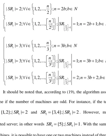
); each problem was considered with two different server constraints as described by (19) and (20).

20 1 2 | | 2; 1, 2,..., ; 2 ; 2 | | 2; 1, 2,..., ; 1; 2 1; 2 i i n n SR i n b b N n SR i SR n b b N        _{  }  _{ }    _{ }       _{       }    _{  } 

(19)

1 3 1 3

|

| 3;

1, 2,...,

;

3 ;

3

|

| 3;

1, 2,...,

;

1;

3

1;

3

|

| 3;

1, 2,...,

;

2;

3

2;

3

i i n i n

n

SR

i

n

b b

N

n

SR

i

SR

n

b

b

N

n

SR

i

SR

n

b

b

N

           









  



















  



 















 



 











 





  











 







 





(20)

It should be noted that, according to (19), the algorithm assigns a dedicated server to the last machine if the number of machines are odd. For instance, if the test problem has 5 machines, then

1

{1,2};|

1

| 2

SR



SR



and

SR

₂



{3,4};|

SR

₂

| 2



. However, machine 5 will be assigned one dedicated server; in other words

SR

₃



{5};|

SR

₃

| 1



. With the same logic, depending on the number of machines, it is possible to have one or two machines instead of three machines assigned to one server, when equation set (20) is in effect. For simplicity, the described conditions of (19) and (20) will be denoted as

SR

2 and

SR

3 throughout the rest of this paper. The proposed GA algorithm was applied to each problem 3 times with 4 different combinations of the parameter values as follows:

Table 3 – Different Parameter Combinations

Parameter Combination 1 Combination 2 Combination 3 Combination 4

Pop

6 n 5 n 2 n

n

m

P

0.2 0.3 0.4 0.5 c P 0.2 0.3 0.4 0.5 l P 0.05 0.1 0.15 0.2

Iter

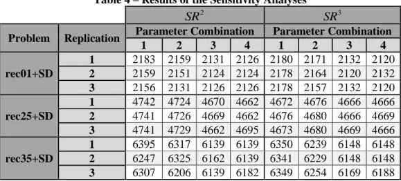
10n 50n 100n 200n

Table 4 presents the resulting makespans for the different combinations of the parameters considered.

21

Table 4 – Results of the Sensitivity Analyses

2

SR SR3

Problem Replication Parameter Combination Parameter Combination

1 2 3 4 1 2 3 4 rec01+SD 1 2183 2159 2131 2126 2180 2171 2132 2120 2 2159 2151 2124 2124 2178 2164 2120 2132 3 2156 2131 2126 2126 2178 2157 2132 2120 rec25+SD 1 4742 4724 4670 4662 4672 4676 4666 4666 2 4741 4726 4669 4662 4676 4680 4666 4669 3 4741 4729 4662 4695 4673 4680 4669 4666 rec35+SD 1 6395 6317 6139 6139 6350 6239 6148 6148 2 6247 6325 6162 6139 6341 6229 6148 6148 3 6307 6206 6139 6182 6349 6254 6169 6188

Analysis of variance (ANOVA) can be utilized to select the best combination from the considered parameter combinations. Considered factors in the ANOVA include parameter combination as defined by table 3, problem set, server constraints, and the interactions between the mentioned factors. In the mentioned ANOVA, each factor has 3 replications. Table 5 summarizes the results of the ANOVA (



0.05).

Table 5 - Analysis of Variance for Makespan Source Degree of Freedom Sequential Sums of Squares Adjusted Sums of Squares Adjusted Mean Square Value F-Value P-Value Problem 2 203814815 203814815 101907407 193904.16 0 Parameter 3 102481 102481 34160 65 0 SR 1 953 953 953 1.81 0.184 Problem*Parameter 6 51672 51672 8612 16.39 0 Problem*SR 2 4898 4898 2449 4.66 0.014 Parameter*SR 3 2035 2035 678 1.29 0.288 Problem*Parameter*SR 6 7349 7349 1225 2.33 0.047 Error 48 25227 25227 526 Total 71 204009429

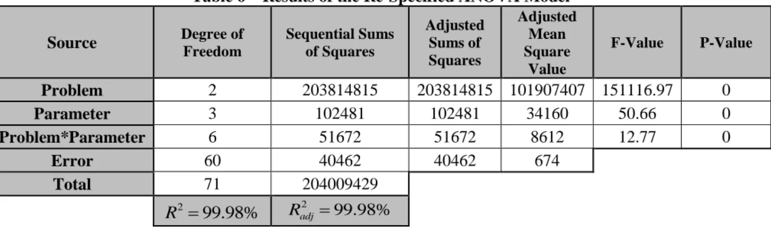
According to the pvalues of table 5, server side constraints are not an important factor in the analysis. Therefore, a re-specification of ANOVA is necessary. Table 6 presents the results of the re-specified model. The importance of the server constraints will be discussed with more details in the following sections.

22

Table 6 – Results of the Re-Specified ANOVA Model Source Degree of Freedom Sequential Sums of Squares

Adjusted Sums of Squares Adjusted Mean Square Value F-Value P-Value Problem 2 203814815 203814815 101907407 151116.97 0 Parameter 3 102481 102481 34160 50.66 0 Problem*Parameter 6 51672 51672 8612 12.77 0 Error 60 40462 40462 674 Total 71 204009429 2 99.98% R  Radj2 99.98%

In order to confirm that the analysis of variance presented in table 6 is valid, residuals should follow a normal distribution. Figure 7 illustrates the normal probability plot of the residuals. To conclude that the residuals follow a normal distribution, they should be close to the normal probability line. Figure 7 confirms that the residuals are very close to the normal line.

Residual P e rc e n t 50 0 -50 -100 99.9 99 95 90 80 70 60 50 40 30 20 10 5 1 0.1

Figure 7 - Normal Probability Plot of the Residuals

As table 6 indicates, the combinations of table 3 have an actual effect on the makespan of the studied test problems. In order to find the best combination among the 4 combinations, the main effects plot proves to be useful. Figure 8 illustrates the main effects plot.

23 Parameter M e a n o f M a k e sp a n 4 3 2 1 4400 4390 4380 4370 4360 4350 4340 4330 4320 4310

Figure 8 - Main Effects Plot

Figure 8 demonstrates that combinations 3 and 4 of table 3 are more desirable than combinations 1 and 2. Since the difference between combinations 3 and 4 is negligible, and combination 3 requires less computational effort, which leads to less CPU time, this combination is chosen for tuning the parameters of both GA and GA+DLS to perform the computational analysis.

The developed algorithms were coded using Microsoft Visual C++ 2008; all the computational experiments were performed on a PC equipped with a 2.66GHz Intel Pentium IV CPU and 4 GB of RAM.

To test the efficiency of the proposed algorithms, a set of 29 problems were chosen from the literature: car01 through car08 introduced by Carlier (1978) and rec01 through rec41 introduced by Reeves (1995). Reeves (1995) found this specific set of problems difficult to solve. Moreover, optimal solutions for the no-wait version of these problems are unknown. All of these test problems are available at OR-Library (Beasley). Samarghandi and ElMekkawy (2014a) generated sequence dependent setups for the problems of Carlier (1978) and Reeves (1995). These problems were named as car+SD and rec+SD, and solved by a PSO algorithm that was designed for

F no wait S

|



,

_sd

|

C

_max. Since

max

, _Q| , _sd|

F S nowait S C is a generalization of

F no wait S

|



,

_sd

|

C

_max, car+SD and rec+SD problems along with server constraints of equations (19) and (20) will be used as test problems in this

24

research. To remain consistent with the literature, each problem is solved 20 times, and the best obtained objective function value as well as the average and worst objective function values are reported. In addition, the average CPU time to obtain the makespans in seconds and standard deviation of the obtained makespans are stated. Section 5.2 reports the computational results of car01 through car08; computational results for rec01 through rec41 appear in section 5.3 and 5.4.

5.2.

Computational Results Obtained for car01 through car08

Table 7 presents the computational results of car01+SD through car08+SD. These problems generally have a lower number of jobs compared to the set of rec+SD problems. As a result, it is possible to solve many of them to optimality by means of the mathematical model of section 3. One can verify that the proposed algorithms are in most cases able to produce the optimal solutions. Tables 8 and 9 report more details about the obtained makespans. Table 8 belongs to SR2 and Table 9 demonstrates the results for SR3.

5.3.

Computational Results of rec01+SD through rec41+SD

Table 10 compares the computational results of the developed algorithms with the makespans generated by the 2-Opt algorithm for problems rec01+SD through rec41+SD. This table considers the case of SR2. It can be verified that both of the developed algorithms are very efficient, with GA+DLS being slightly better than GA. Small values of the STD column is another indicator of the consistency of the proposed PSO. Table 11 performs the same comparison for the case of SR3. Section 5.4 compares the results of the developed algorithms for F S, _Q|nowait S, _sd|C_max with the results of Samarghandi and ElMekkawy (2014a) for

F no wait S

|



,

_sd

|

C

_max.

5.4.

Comparison of the Solutions of

F S, _Q|nowait S, _sd|C_max

with

max

|

,

_sd

|

F no wait S



C

Table 12 performs a comparison between the results of Samarghandi and ElMekkawy (2014a)

25

Table 7 – Computational Results for Problems with Optimal Solution

Problem

n m

,

No Server Constraint Optimal Solution for SR2 Optimal Solution for SR3 GA - SR2 GA+DLS - SR2 GA - SR3 GA+DLS - SR3

OFV* OFV OFV Best

Solution Gap** Best Solution Gap Best Solution Gap Best Solution Gap Car01+SD 11,5 10,379.00 10,379.00 10,402.00 10,379.00 100.000 10,379.00 100.000 10,402.00 100.000 10,402.00 100.000

Car02+SD 13,4 N/A N/A N/A 11,486.00 N/A 11,486.00 N/A 11,488.00 N/A 11,488.00 N/A

Car03+SD 12,5 11,877.00 11,877.00 11,919.00 11,877.00 100.000 11,877.00 100.000 11,919.00 100.000 11,919.00 100.000

Car04+SD 14,4 N/A N/A N/A 12,384.00 N/A 12,384.00 N/A 12,398.00 N/A 12,398.00 N/A

Car05+SD 10,6 11,945.00 12,068.00 12,266.00 12,068.00 100.000 12,068.00 100.000 12,270.00 100.033 12,266.00 100.000

Car06+SD 8,9 12,015.00 12,131.00 12,131.00 12,131.00 100.000 12,131.00 100.000 12,131.00 100.000 12,131.00 100.000

Car07+SD 7,7 9,795.00 9,815.00 9,795.00 9,815.00 100.000 9,815.00 100.000 9,795.00 100.000 9,795.00 100.000

Car08+SD 8,8 11,525.00 11,525.00 11,684.00 11,525.00 100.000 11,525.00 100.000 11,684.00 100.000 11,684.00 100.000

* Objective Function Value

** Algorithm

Optimal

100

OFV

26

Table 8 – Detailed Computational Results for the Case of SR2

Problem

n m

,

2-Opt OFV* GA GA+DLS Best OFV Average OFV Worst OFV STD** CPU Time Gap*** Best OFV Average OFV Worst OFV STD CPU Time Gap car01+SD 11,5 14,830.00 10,379.00 10,401.10 10,647.00 58.76 8.14 69.99% 10,379.00 10,437.33 10,909.00 60.14 10.58 69.99% car02+SD 13,4 15,290.00 11,486.00 11,584.65 11,674.00 62.51 8.44 75.12% 11,486.00 11,654.55 11,936.00 61.78 10.97 75.12% car03+SD 12,5 15,898.00 11,877.00 11,984.55 12,174.00 92.76 8.41 74.71% 11,877.00 11,985.88 12,346.00 65.39 10.93 74.71% car04+SD 14,4 16,571.00 12,384.00 12,616.05 12,865.00 146.48 8.33 74.73% 12,384.00 12,561.98 12,930.00 82.89 10.66 74.73% car05+SD 10,6 15,383.00 12,068.00 12,109.55 12,546.00 129.49 8.44 78.45% 12,068.00 12,138.15 12,552.00 69.60 10.80 78.45% car06+SD 8,9 15,623.00 12,131.00 12,255.60 12,590.00 179.07 9.93 77.65% 12,131.00 12,281.18 12,590.00 103.29 12.71 77.65% car07+SD 7,7 12,579.00 9,815.00 9,834.80 9,944.00 42.90 7.42 78.03% 9,815.00 9,837.20 9,944.00 35.55 9.50 78.03% car08+SD 8,8 14,099.00 11,525.00 11,545.70 11,606.00 26.78 8.53 81.74% 11,525.00 11,543.23 11,597.00 20.19 10.91 81.74%

Average N/A N/A N/A N/A N/A 92.34 8.45 76.30% N/A N/A N/A 62.35 10.88 76.30%

* Objective Function Value **Standard Deviation

*** Algorithm

2-Opt

100

Best OFV

27

Table 9 – Detailed Computational Results for the Case of SR3

Problem

n m

,

2-Opt OFV* GA GA+DLS Best OFV Average OFV Worst OFV STD** CPU Time Gap*** Best OFV Average OFV Worst OFV STD CPU Time Gap car01+SD 11,5 13,111.00 10,402.00 10,429.60 10,542.00 40.99 8.34 79.34% 10,402.00 10,417.58 10,623.00 43.57 10.93 79.34% car02+SD 13,4 15,212.00 11,488.00 11,558.45 11,695.00 66.93 8.13 75.52% 11,488.00 11,618.53 12,023.00 113.00 10.64 75.52% car03+SD 12,5 17,733.00 11,919.00 12,016.90 12,080.00 57.55 8.42 67.21% 11,919.00 12,067.90 12,360.00 103.06 11.19 67.21% car04+SD 14,4 15,784.00 12,398.00 12,588.75 12,905.00 156.56 8.50 78.55% 12,398.00 12,596.18 12,846.00 124.55 11.31 78.55% car05+SD 10,6 15,550.00 12,270.00 12,395.15 12,559.00 112.06 8.54 78.91% 12,266.00 12,305.65 12,558.00 65.59 11.02 78.88% car06+SD 8,9 15,814.00 12,131.00 12,358.95 12,590.00 233.88 9.69 76.71% 12,131.00 12,226.45 12,590.00 162.99 12.49 76.71% car07+SD 7,7 12,846.00 9,795.00 9,799.70 9,889.00 21.02 7.49 76.25% 9,795.00 9,811.45 9,889.00 36.17 9.59 76.25% car08+SD 8,8 14,607.00 11,684.00 11,703.45 11,857.00 39.83 8.66 79.99% 11,684.00 11,727.78 12,022.00 86.29 11.09 79.99%

Average N/A N/A N/A N/A N/A 91.10 8.47 76.56% N/A N/A N/A 91.90 11.03 76.56%

* Objective Function Value **Standard Deviation

*** Algorithm

2-Opt

100

Best OFV

28

Table 10 – Detailed Computational Results for the Case of SR2

Problem

n m

,

2-Opt OFV* GA GA+DLS Best OFV Average OFV Worst OFV STD** CPU Time Gap*** Best OFV Average OFV Worst OFV STD CPU Time Gap rec01+SD 20,5 2,822.00 2,124.00 2,144.15 2,183.00 14.28 11.82 75.27% 2,118.00 2,145.58 2,183.00 16.51 15.12 75.05% rec03+SD 20,5 2,824.00 1,911.00 1,929.30 1,973.00 14.53 11.99 67.67% 1,884.00 1,930.15 1,987.00 27.14 15.35 66.71% rec05+SD 20,5 2,902.00 2,007.00 2,046.80 2,090.00 22.71 11.72 69.16% 2,010.00 2,041.70 2,090.00 18.25 15.00 69.26% rec07+SD 20,10 3,764.00 2,649.00 2,682.85 2,764.00 32.68 19.25 70.38% 2,637.00 2,682.33 2,741.00 30.36 24.63 70.06% rec09+SD 20,10 3,655.00 2,660.00 2,695.80 2,757.00 21.44 19.22 72.78% 2,675.00 2,695.03 2,741.00 15.49 24.60 73.19% rec11+SD 20,10 3,205.00 2,571.00 2,586.50 2,632.00 16.59 19.41 80.22% 2,565.00 2,588.55 2,617.00 13.32 23.48 80.03% rec13+SD 20,15 4,387.00 3,315.00 3,352.15 3,437.00 26.68 25.43 75.56% 3,324.00 3,355.25 3,401.00 15.43 30.76 75.77% rec15+SD 20,15 4,330.00 3,253.00 3,277.85 3,322.00 22.75 25.87 75.13% 3,237.00 3,272.80 3,328.00 26.12 31.30 74.76% rec17+SD 20,15 4,219.00 3,274.00 3,309.15 3,361.00 28.24 25.10 77.60% 3,271.00 3,291.43 3,337.00 17.61 30.36 77.53% rec19+SD 30,10 5,401.00 3,867.00 3,887.25 3,917.00 15.97 32.64 71.60% 3,851.00 3,901.63 3,971.00 29.04 39.49 71.30% rec21+SD 30,10 4,980.00 3,743.00 3,776.95 3,824.00 23.54 32.77 75.16% 3,714.00 3,748.75 3,832.00 29.48 43.26 74.58% rec23+SD 30,10 5,507.00 3,623.00 3,652.30 3,730.00 32.36 31.37 65.79% 3,587.00 3,664.15 3,725.00 26.15 41.40 65.14% rec25+SD 30,15 6,094.00 4,662.00 4,708.85 4,768.00 32.03 43.47 76.50% 4,644.00 4,695.03 4,763.00 33.08 57.38 76.21% rec27+SD 30,15 6,348.00 4,562.00 4,611.65 4,673.00 27.17 42.99 71.87% 4,550.00 4,589.60 4,620.00 16.33 56.75 71.68% rec29+SD 30,15 6,172.00 4,443.00 4,483.90 4,524.00 24.38 42.47 71.99% 4,424.00 4,475.20 4,544.00 32.69 56.05 71.68% rec31+SD 50,10 8,919.00 5,936.00 6,029.60 6,129.00 51.98 100.63 66.55% 5,911.00 6,021.28 6,176.00 64.09 127.90 66.27% rec33+SD 50,10 8,917.00 6,159.00 6,211.90 6,352.00 45.00 99.48 69.07% 6,155.00 6,225.10 6,294.00 30.13 126.44 69.03% rec35+SD 50,10 9,329.00 6,139.00 6,251.05 6,395.00 73.33 100.31 65.81% 6,143.00 6,196.53 6,314.00 39.41 127.49 65.85% rec37+SD 75,20 15,841.00 10,985.00 11,076.60 11,177.00 45.60 604.32 69.35% 10,957.00 11,059.95 11,191.00 61.88 742.70 69.17% rec39+SD 75,20 16,783.00 11,299.00 11,401.05 11,503.00 68.17 597.69 67.32% 11,303.00 11,450.05 11,701.00 93.80 734.55 67.35% rec41+SD 75,20 16,428.00 11,494.00 11,579.60 11,692.00 65.39 605.11 69.97% 11,461.00 11,528.53 11,623.00 42.58 743.67 69.77% Average NA NA NA NA NA 33.56 119.19 71.65% NA NA NA 32.33 147.99 71.45%

* Objective Function Value **Standard Deviation

*** Algorithm

2-Opt

100

Best OFV

29

Table 11 – Detailed Computational Results for the Case of SR3

Problem

n m

,

2-Opt OFV* GA GA+DLS Best OFV Average OFV Worst OFV STD** CPU Time Gap*** Best OFV Average OFV Worst OFV STD CPU Time Gap rec01+SD 20,5 2,880.00 2,120.00 2,144.35 2,180.00 18.75 11.88 73.61% 2,125.00 2,148.60 2,188.00 17.08 15.22 73.78% rec03+SD 20,5 2,826.00 1,890.00 1,916.30 1,950.00 17.02 12.64 66.88% 1,880.00 1,922.05 1,965.00 21.59 16.19 66.53% rec05+SD 20,5 2,663.00 2,032.00 2,057.60 2,110.00 23.92 13.03 76.30% 2,010.00 2,048.20 2,129.00 24.09 16.69 75.48% rec07+SD 20,10 3,609.00 2,671.00 2,711.75 2,752.00 20.04 19.99 74.01% 2,671.00 2,698.95 2,772.00 22.48 26.18 74.01% rec09+SD 20,10 3,392.00 2,644.00 2,674.35 2,714.00 16.70 19.34 77.95% 2,669.00 2,691.08 2,739.00 17.77 25.34 78.69% rec11+SD 20,10 3,538.00 2,600.00 2,628.65 2,665.00 20.52 19.02 73.49% 2,599.00 2,619.25 2,659.00 14.56 24.91 73.46% rec13+SD 20,15 4,337.00 3,343.00 3,374.10 3,422.00 21.40 26.77 77.08% 3,319.00 3,359.63 3,411.00 27.24 35.07 76.53% rec15+SD 20,15 4,602.00 3,257.00 3,307.45 3,326.00 15.95 27.00 70.77% 3,242.00 3,279.03 3,316.00 22.96 35.90 70.45% rec17+SD 20,15 4,390.00 3,267.00 3,296.75 3,320.00 18.78 27.34 74.42% 3,268.00 3,287.08 3,326.00 16.33 36.36 74.44% rec19+SD 30,10 5,546.00 3,871.00 3,927.30 3,984.00 31.29 34.27 69.80% 3,812.00 3,886.10 3,987.00 34.57 45.57 68.73% rec21+SD 30,10 5,033.00 3,781.00 3,804.90 3,851.00 19.96 33.05 75.12% 3,729.00 3,786.53 3,835.00 25.35 43.96 74.09% rec23+SD 30,10 5,645.00 3,658.00 3,702.75 3,739.00 23.21 33.59 64.80% 3,634.00 3,682.30 3,730.00 24.93 44.67 64.38% rec25+SD 30,15 6,456.00 4,666.00 4,676.40 4,689.00 6.28 45.83 72.27% 4,659.00 4,687.15 4,752.00 22.18 59.17 72.17% rec27+SD 30,15 6,615.00 4,622.00 4,646.65 4,689.00 17.25 46.53 69.87% 4,559.00 4,608.18 4,650.00 25.65 60.06 68.92% rec29+SD 30,15 6,339.00 4,458.00 4,493.25 4,538.00 20.73 46.38 70.33% 4,452.00 4,514.23 4,623.00 37.35 59.87 70.23% rec31+SD 50,10 8,785.00 5,957.00 6,005.10 6,185.00 69.57 101.90 67.81% 5,931.00 6,029.98 6,096.00 42.44 131.55 67.51% rec33+SD 50,10 8,970.00 6,183.00 6,231.20 6,310.00 33.65 101.70 68.93% 6,178.00 6,237.03 6,286.00 24.18 131.29 68.87% rec35+SD 50,10 9,812.00 6,148.00 6,306.10 6,389.00 83.23 100.41 62.66% 6,169.00 6,242.55 6,351.00 44.46 129.63 62.87% rec37+SD 75,20 15,066.00 10,861.00 10,954.20 11,011.00 37.50 633.81 72.09% 10,881.00 11,000.13 11,093.00 63.28 842.96 72.22% rec39+SD 75,20 16,402.00 11,328.00 11,387.05 11,463.00 40.98 921.74 69.06% 11,296.00 11,415.30 11,510.00 53.37 1,015.75 68.87% rec41+SD 75,20 16,952.00 11,450.00 11,536.85 11,598.00 35.91 634.87 67.54% 11,441.00 11,565.83 11,789.00 99.29 768.19 67.49% Average NA NA NA NA NA 28.22 138.62 71.18% NA NA NA 32.44 169.74 70.94%

* Objective Function Value **Standard Deviation

*** Algorithm

2-Opt

100

Best OFV

30

Table 12 – Comparison of the Results of Samarghandi and ElMekkawy (2014a) for

F no wait S

|



,

_sd

|

C

_max with the Results of the Developed Algorithms for F S, _Q|nowait S, _sd|C_max

Problem

n m

,

No Server Constraint

OFV*

GA - SR2 GA - SR3 GA+DLS - SR2 GA+DLS - SR3

OFV Gap** OFV Gap OFV Gap OFV Gap

rec01+SD 20,5 2,139.00 2,124.00 99.29874 2,120.00 99.11173 2,118.00 99.01823 2,125.00 99.34549 rec03+SD 20,5 1,902.00 1,911.00 100.47319 1,890.00 99.36909 1,884.00 99.05363 1,880.00 98.84332 rec05+SD 20,5 2,028.00 2,007.00 98.96450 2,032.00 100.19724 2,010.00 99.11243 2,010.00 99.11243 rec07+SD 20,10 2,652.00 2,649.00 99.88688 2,671.00 100.71644 2,637.00 99.43439 2,671.00 100.71644 rec09+SD 20,10 2,657.00 2,660.00 100.11291 2,644.00 99.51073 2,675.00 100.67746 2,669.00 100.45164 rec11+SD 20,10 2,558.00 2,571.00 100.50821 2,600.00 101.64191 2,565.00 100.27365 2,599.00 101.60281 rec13+SD 20,15 3,309.00 3,315.00 100.18132 3,343.00 101.02750 3,324.00 100.45331 3,319.00 100.30221 rec15+SD 20,15 3,222.00 3,253.00 100.96214 3,257.00 101.08628 3,237.00 100.46555 3,242.00 100.62073 rec17+SD 20,15 3,271.00 3,274.00 100.09172 3,267.00 99.87771 3,271.00 100.00000 3,268.00 99.90828 rec19+SD 30,10 3,848.00 3,867.00 100.49376 3,871.00 100.59771 3,851.00 100.07796 3,812.00 99.06445 rec21+SD 30,10 3,756.00 3,743.00 99.65389 3,781.00 100.66560 3,714.00 98.88179 3,729.00 99.28115 rec23+SD 30,10 3,628.00 3,623.00 99.86218 3,658.00 100.82690 3,587.00 98.86990 3,634.00 100.16538 rec25+SD 30,15 4,654.00 4,662.00 100.17190 4,666.00 100.25784 4,644.00 99.78513 4,659.00 100.10743 rec27+SD 30,15 4,565.00 4,562.00 99.93428 4,622.00 101.24863 4,550.00 99.67141 4,559.00 99.86857 rec29+SD 30,15 4,422.00 4,443.00 100.47490 4,458.00 100.81411 4,424.00 100.04523 4,452.00 100.67843 rec31+SD 50,10 5,966.00 5,936.00 99.49715 5,957.00 99.84915 5,911.00 99.07811 5,931.00 99.41334 rec33+SD 50,10 6,186.00 6,159.00 99.56353 6,183.00 99.95150 6,155.00 99.49887 6,178.00 99.87068 rec35+SD 50,10 6,169.00 6,139.00 99.51370 6,148.00 99.65959 6,143.00 99.57854 6,169.00 100.00000 rec37+SD 75,20 10,782.00 10,985.00 101.88277 10,861.00 100.73270 10,957.00 101.62308 10,881.00 100.91820 rec39+SD 75,20 11,189.00 11,299.00 100.98311 11,328.00 101.24229 11,303.00 101.01886 11,296.00 100.95630 rec41+SD 75,20 11,324.00 11,494.00 101.50124 11,450.00 101.11268 11,461.00 101.20982 11,441.00 101.03320 Average NA NA NA 100.28248 NA 100.59481 NA 100.06922 NA 100.34411

* Objective Function Value

** Al