ISSN: 1992-8645 www.jatit.org E-ISSN: 1817-3195
SENSITIVITY ANALYSIS OF CREW SKILL TO
MAINTENANCE COST AND RELIABILITY FOR MAIN
ENGINE SUPPORT SYSTEMS USING SYSTEM
DYNAMICS
1DIDIET SUDIRO RESOBOWO 2LAHAR BALIWANGI, KETUT BUDA ARTANA, AAB
DINARIYANA
1Graduate School of Marine Technology ITS Surabaya
2Reliability and Safety Laboratory, Department of Marine Engineering ITS
Campus ITS, Surabaya 60111
E-mail: 1
[email protected]
, 2[email protected]ABSTRACT
System operation and maintenance always depends on system components’ characteristic. Further, components which build a system yield unique system behaviors beside the components operation and maintenance condition. The objective of paper presented here is to identify and understand behavior of component and as well behavior of system under various operation and maintenance policies and to understand the sensitivity of crew skill in determining the reliability and maintenance policy. The model developed here can be directed to give maintenance policy options to the management as decision maker and further, to provide picture on impacts of those options. This work presents a user friendly and easy model to simulate the effect of various operation and maintenance plans to the system reliability, operation cost, and maintenance cost, as well as the sensitivity of crew skill in affecting the maintenance schedule and the system reliability. For each plan of operation and maintenance, this simulation models failure rate, time to maintain, decision whether to maintain or not, degree of how good maintenance done, effect of component after maintenance to the system, maintenance cost, and operation cost. A case study of main engine cooling system is presented using previous works data [1]. The simulation shows prognostic results for a given scenario of system configuration, operation, and maintenance plan.
Keywords: System Dynamic, Ship Maintenance, Crew Skill, Reliability, Maintenance Cost
1. BACKGROUND
System dynamics (SD) concerns a system’s dynamic behavior over time under various conditions. SD is designed to investigate cause-effect relationships among equipments as well as the characteristic and functions of a complex system. Through this better understanding, a conscious learning on interaction among components in a system could help decision maker of doing operation and/or maintenance of component and system.
Dependence of a system reliability and performance to the way of operation and maintenance management is absolutely certain. Two identical systems or components might not give the same performance in different treatment and different operating condition. System reliability certainly related to operating time period, failure rate of each component, and restore rate of maintenance. Whilst total expenses is affected by
performance loss caused by lack of maintenance, maintenance cost, and earning loss.
Further, maintenance strategy and system performance, especially for marine systems, is heavily affected by the skill of maintenance engineer (crew skill). The affect of the crew skill, however, is hardly defined. This paper tries to model the unknown behavior of inter-relation between crew skill, reliability and maintenance schedule using SD, by representing them as a cause-effect relationship linking among components in a system. In such a way, a better understanding of system behavior can be expected, and further, a better operation and maintenance management could be reached by a better understanding of system behavior.
2. LOGIC OF CAUSE-EFFECT DESIGN
to correspond to what is, or might be happening, in real world. SD is relatively close to the system thinking (ST) which produces causal-loop flow to illustrate common behavior while SD itself translates the understanding gained by ST into a computer simulation model [6].
SD works based on the principle of cause-effect with feedback and/or delay depends on the complexity of system [7]. The idea is that actions and decisions result consequences. When actions and decisions change, the consequences will also change. Therefore, we can simulate any possible consequence of system operation and maintenance decisions we plan to take.
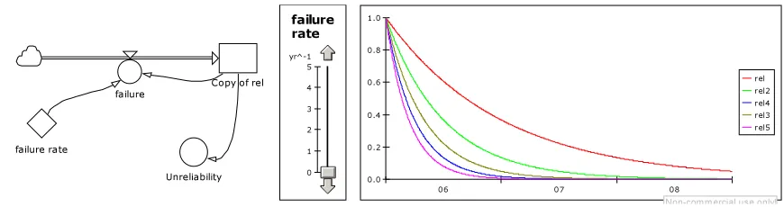
Figure 1 shows a causal relationship diagram of a component behavior. The component behavior could be explained with its reliability and performance. The reliability and performance are dynamic since in general, they reduce or possibly increase with time and always depend on other related factors such as environment condition, operation condition, and maintenance. The crew skill will directly affect the restore rate, and inherently also affect the failure rate of the components. The reliability causal relationship
diagram above can be illustrated in a simple SD model as shown in figure 2.
From the model, by shifting the failure rate bar (in the middle), SD will present different component reliability over time (right side). This will inform us the probability of component survival given times. Therefore, decision whether to maintain or not then also can be determined or simulated after reaching a certain minimum level of reliability.
3. MODEL DEVELOPMENT FOR A MAIN
ENGINE FUEL OIL SYSTEM
Let us define T is random time of a component failure then the distribution of failure or recognized as unreliability function given by,
∫
>= ≤ =
t
t for du u f t T P t F
0
0 ) ( ) ( )
( (1)
Reliability function R(t) represents the probability that a component does not fail within a certain time interval (0,t), it can be expressed as,
0 ) ( ) ( 1 )
(t = −F t =PT>t for t>
[image:2.595.87.511.429.569.2]R (2)
Figure 1. Reliability And Performance Causal Relationship Diagram
06 07 08
0.0 0.2 0.4 0.6 0.8 1.0
rel rel2 rel4 rel3 rel5
Non-comm ercial use only! failure
rate
0 1 2 3 4 5 yr^-1
failure
Copy of rel
failure rate
[image:2.595.79.514.594.709.2]Unreliability
ISSN: 1992-8645 www.jatit.org E-ISSN: 1817-3195
A system configuration could either be a series, parallel, series-parallel, parallel-series, k out of n, redundant, or even complex configuration. Following is a short discussion of system configurations reliability modeling: series and parallel configuration.
Series configuration:
[image:3.595.99.279.279.307.2]The series configuration is the simplest configuration and the most commonly used in practice. The block diagram of series configuration and parallel configuration is given in figure 3.
Figure 3. A Series Configuration
For this configuration, all components must be operating to assure system operation. The system fails if one of the components fails. If Pr(Ei) is probability of an event Ei that component i operates successfully during a certain period of time thus reliability function of a series configuration is given by,
Rs = Pr (all components operate successfully)
∏
= − = ∩ ∩ ∩ = n i i s n n s E R E E E E R 1 1 2 1 ) Pr( ) ... Pr(Therefore, when assumed that each component operates independently, the system reliability for series configuration could be expressed by,
∏
= = n i i s R R 1 (3)Where Ri is reliability of component i.
[image:3.595.97.513.469.739.2]Parallel configuration:
Figure 4. A parallel configuration
For parallel configuration, system fails if all components fail. In other words, system will successfully operate if any component performs its function. Thus, probability of parallel configuration being success is union probability of all paralleled component which can be written as,
Rs = Pr (any components operate successfully) )
...
Pr( 1 2 n1 n
p E E E E
R = ∪ ∪ − ∪
) ...
Pr(
1 1 2 n 1 n
p E E E E
R = − ∩ ∩ − ∩
If the probability of failure (unreliability) of a single component is expressed with Q, then
∏
= − = − = n i i pp Q Q
R
1
1
1
(4)
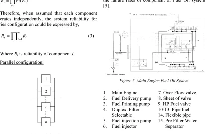
A main engine Fuel Oil system is taken as a case study in this research. The main engine Fuel Oil system shown in figure 5, Fuel Oil is pumped from base tank to daily tank using pre-filter with water separator to separate the impurities contained in the Fuel Oil, further from the daily tank supply were bought to the duplex filters selectable by the fuel oil delivery pump to the fuel oil injectors, the remaining fuel oil is returned to basis tank through the overflow valve, the next process repeated as before.
Data used for this case study, given in table 1, are the failure rates of component of Fuel Oil system [5].
Figure 5. Main Engine Fuel Oil System
1. Main Engine. 2. Fuel Delivery pump 3. Fuel Priming pump 4. Duplex Filter
Selectable
5. Fuel injection pump 6. Fuel injector
7. Over Flow valve. 8. Sheet of valve 9. HP Fuel valve 10-13. Pipe fuel 14. Flexible pipe 15. Pre Filter Water
Separator
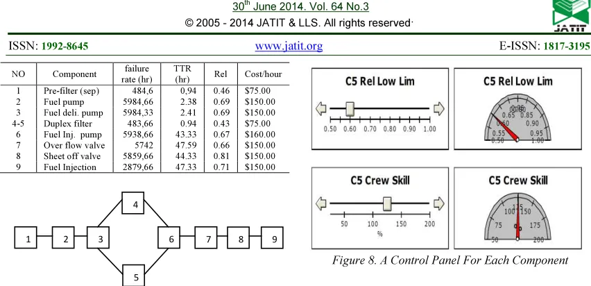
Table1: Components, Failurerate, TTR, Reliability, Cost.
1
2
i
n
Failure Rate-1
0.0 0.5 1.0 1.5 2.0 yr ^ -1
Restore rate-1
4.0 4.5 5.0 5.5 6.0 yr ^ -1
NO Component rate (hr) failure TTR (hr) Rel Cost/hour
1 Pre-filter (sep) 484,6 0,94 0.46 $75.00
2 Fuel pump 5984,66 2.38 0.69 $150.00
3 Fuel deli. pump 5984,33 2.41 0.69 $150.00
4-5 Duplex filter 483,66 0.94 0.43 $75.00
6 Fuel Inj. pump 5938,66 43.33 0.67 $160.00
7 Over flow valve 5742 47.59 0.66 $150.00
8 Sheet off valve 5859,66 44.33 0.81 $150.00
9 Fuel Injection 2879,66 47.33 0.71 $150.00
1 2 3 6 7 8 9
[image:4.595.82.508.82.288.2]5 4
Figure 6a. Reliability Block Diagram, Fuel Oil System
The system Reliability then is expressed mathematically using equation (1-4). The Equation is used for final calculation formula in an auxiliary of SD; placed in a black auxiliary in Figure 6b. Data used for this case study given in table 1, are the failure rates of component of fuel oil system [1].
1 2 3 4 5 6 7 8 9 101112 0.0
0.2 0.4 0.6 0.8 1.0
With Mainten an ce Withou t M ain tenance
R
e
li
a
b
il
it
y
L
e
v
e
[image:4.595.88.284.395.493.2]l
Figure 7. An Example Of Reliability Plot Of A Component With And Without Maintenance
Figure 8. A Control Panel For Each Component
When the simulation is run by time, condition of each component can be set either run or maintain, as shown in figure 8. If “run” is set, the failure rate reduces reliability. At the same time there is no additional cost but performance loss. When “maintain” is set, restore rate is applied to the component and reliability of component will increase and the performance as well, but it increases the maintenance cost. On the other plan scenario, “maintain” mode for each component could also be set as periodical maintenance (for example, every three months) using command time cycle of the SD program. The model could also be able to relate the failure effect of one component to other component(s) if it is set. That means the model could state that no component is independent. To relate the failure effect among components, previous studies result could be utilized [6].
C1 Rate
C1 Reliability
C1 Failure rate
C1 Exponential
C1 Lamda C1 Time step
C1 Op Time
C1 Operate C1 Condition C1 Maintain C1 Rel Low Lim
C1 Rel Up Lim C1 Failure_rate
C1 Total Maint Cost C1 Labor Cost
C1 Mnt cost per hr C1 TTM
C1 Tot Consequence C1 Tot Loss
C1 Loss C1 loss rate
C1 Risk
C1 Reset
C1 control
C1 return
C1 Crew Skill
C1 Skill Factor To TTM
C1 Skill Factor to Cost CSkill
Low est R
LaborCost
LossRate
[image:4.595.175.434.522.719.2]ISSN: 1992-8645 www.jatit.org E-ISSN: 1817-3195
Figure 8 is the control panel for each component. This control panel is to control the characteristic of component based on the historical data, operation data, and/or reliability value. In addition, decision when to operate or to maintain is also controlled from this control panel. The simulation results: system reliability, performance loss, earning loss and maintenance cost are then obtained after simulation for given certain scenarios. Therefore, operation and maintenance plan could be easily simulated using system dynamics in seeking the best plan based on safety and economic point of view.
4. SENSITIVITY OF CREW SKILL TO MAINTENANCE COST AND SYSTEM PERFORMANCE
Relationship between reliability level and performance might not be able to be defined clearly. However, in general, reducing reliability will always be followed by performance loss because reducing reliability level caused by aging factor, wear out, lack of maintenance, etc., also result performance loss, Reliability plot of a component with and without maintenance. It is illustrated in figure 7.
The question will then come up on how the crew skill will affect the system performance (reliability) and its maintenance strategy (schedule) To enable analyze it, the existing SD model is then further developed by varying the crew skill (incrementing
by certain percentage to the current skill of 100%) and examine its implication to cost (maintenance cost) at various level of reliability.
As shown in 9, SD model is developed by integrating 9 components. The reliability of each component is analyzed at a certain time increment and when the reliability index reaches the minimum allowable limit then the component will be maintained at a certain time to maintenance (TTM). The TTM will be very much depending upon the skill of maintenance crew and the existing condition is set to be 100%. Better crew skill requires less TTM. The simulation if set for a time duration of 1 year.
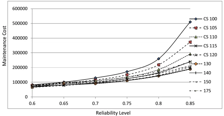
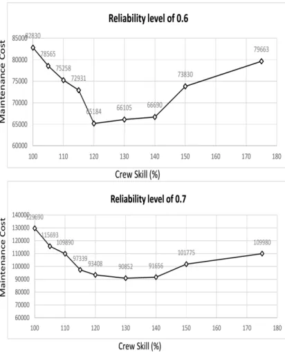
[image:5.595.110.487.505.700.2]Figure 10 shows the result of SD Simulation of effect of crew skill to maintenance cost at various reliability levels. As shown, the increase of crew skill can be perfectly simulated in affecting the increase of consequence (maintenance cost) at a certain reliability level. It means that policy in enhancing the skill of maintenance engineers will reduce the maintenance cost and at the same time, the increase of reliability requirement (level) at a certain crew skill will directly affect the cost of investment (due to utilization of higher quality components) and cost of maintenance (due to more frequent maintenance). Considering the fact, it would then very much necessary to examine the extent of increase of crew skill that finally provide the minimum cost.
672
Figure 10. Crew Skill Vs Maintenance Cost
Figure 11. Effect Of Crew Skill To Maintenance Cost
Having simulated the SD model to a simulation time of 1 year, it is found that the maintenance cost is significantly affected by the crew skill, as shown in Figure 10. For all minimum level of required reliability index (LL 0.6 to LL 0.8), the minimum maintenance cost is obtained at various crew skills. In general, however, it is clearly a certain level of
crew skill improvement required to provide the minimum maintenance cost for each level of reliability index.
Figure 11shows a clearer picture of the above result obtained by comparing two levels of reliability index. At a required level of reliability of 0.6, the increase of crew skill of 20% to the current condition (at 120%) results in the minimum maintenance cost. This means that with regards to system complexity, skill improvement of more than 20% will give no additional advantage in reducing the maintenance cost. The same situation is also shown when the required reliability level is set to 0.7, and then the minimum cost is found at 30% of crew skill improvement. In general we can also see the picture that increase of system complexity requires more skillful crew as well as more investment through skill improvement program.
5. CONCLUSIONS
The simulation shows prognostic results for a given scenario of system configuration, operation and maintenance management. Using SD simulation, the behavior of each component and integrated system could be studied. Further, operation and maintenance activity contribute to the performance could also be simulated with SD. Therefore, it informs the management the best way of operation and maintenance.
[image:6.595.88.294.369.624.2]ISSN: 1992-8645 www.jatit.org E-ISSN: 1817-3195
is existed. However, it is valuable to understand the extent of crew skill improvement to manage the assets that eventually provide technical and economical benefit. Unmeasured program in improving the crew skill does not necessarily provide best solution without considering the complexity of the managed system.
REFERENCES:
[1] Artana KB, Ishida K, ‘Spreadsheet Modeling of Optimal Maintenance Schedule for Components in Wear-Out Phase’, Journal of Reliability Engineering and System Safety, ELSEVIER, Vol. 77 pp. 81-91, 2002.
[2] Artana KB, Ishida K, “Optimum replacement and Maintenance Scheduling Process for Marine Machinery in wear out period”, 3rd New Ship and Marine Technology. pp.111-120 [3] Artana KB, Ishida K, “Optimum replacement and Maintenance Scheduling Process for Marine Machinery in wearout Phase A Chase Study of Main Engine Cooling Pumps”,
Reliability Engineering and Safety
200.81(2002) p.81-91
[4] Baliwangi L.et al, “Otimizing Ship Machinery Maintenance Scheduling Trough Risk And Life cycle Cost”, 25th International Conferency on Offshore Machanic and Artic
Engineering 2006 Hamburg Germany
[5] Baliwangi L.et al, “Risk Modification Through System Dynamics Simulation”
Modelling and Simulation 2007, Mountreal PC Canada ACTAPRESS
[6] Baliwagi L., et al. “Research on marine Incidents Trend in Indonesia 2001 to 2004”,
Japan society for The Promotion of Science
International Seminar in Marine
Transportation 2005, Hiroshima: JSPS [7] Artana KB, Ishida K, “Spreadsheet Modeling
to Determine Optimum Ship Main Dimensions and Power Requirements at Basic Design Stage”, Journal of Marine Technology
Vol. 40 No. 1, Society of Naval Architects and Marine Engineers (SNAME), January 2003. [8] Baliwangi L “Risk and Life Cycle Cost Based
Assessment”, Multi Obyective Simulation Of Ship Machinery Maintenance.
[9] Baliwagi, L Arina, Artana KB, Ishida K (2007), “System Dynamic Simulation For Assigning Operation and Maintenance Management”.
[10] Artana KB, Ishida K (2001). “Determination of ship machinery performance and its maintenance management scheme using
MARKOV process analysis”. Marine Technology IV, WIT Press: 379-389
[11] Pham, Hoang and Wang, Hongzhou, “Imperfect maintenance”, European Journal of Operational Research 94 (1996) 425-438 [12] Reliability Analysis Centre, Non-Electronic