An Analysis on Mammograms using KDA in Multi
Transform Domain
B. N. Prathibha
Assistant Professor, National Engineering College,
Kovilpatti
ABSTRACT
Developing a robust Computer Aided Diagnosis (CADx) system for mammograms analysis has been the challenging task for years. The slight difference in X-ray attenuation between normal and abnormal glandular tissues makes the mammogram diagnosis complicated. The proposed CAD system discriminates the abnormal severity of mammograms into benign (non-cancerous, non-spreadable), normal-malign (cancerous) ans benign-,normal-malign, using wavelet features combined with spectral domain. Classification is performed on 206 different mammogram images from Mias database using Kernel Discriminant Analysis (KDA). KDA affords a non-parametric statistical approach with parzen window density estimation to estimate density function from a given sample dataset. The study reveals that the optimal smoothing parameters are increasing functions of the sample size of the complementary classes, features used to classify and value of the bandwidth.
Keywords
Transforms, Mammograms, KDA, Accuracy, MCC
1.
INTRODUCTION
Breast cancer is one of the leading causes of mortality in women population. Mammography is a crucial X-ray examination technique that photographs the inside tissue abnormalities of the breast. It is one of the best screening methods used for early detection of breast cancer for decades. Mammography detects lumps that are often too small or too deep to feel. If cancer is detected earlier, the patient’s chances are better for a favorable outcome. Early detection of the cancer leads to significant improvements in conservative treatment. Varieties of CADx are developed in order to improve the accuracy of interpretation. Through the combination of digital Mammography and CADx, radiologists can give better diagnostics that will positively impact millions of women. CADx’s have the potential to detect findings that might otherwise be overlooked during the review process, thus increasing cancer detection. Thus the need for "callbacks" or "repeat mammograms" is greatly diminished, if not eliminated.
The proposed methodology studies the performance of the KDA classifier using wavelet features with spectral domain for discriminating breast tissues into normal and benign, normal and malign, benign and malignant. The original mammogram is transformed into spectral domain, the resultant image coefficients are merged with features obtained after sub sampling with discrete wavelet transform (DWT).
The extracted feature sets are evaluated by means of their ability in differentiating the severity of the breast cancer using the KDA classification algorithm. The performance of different filters as well as the efficiency of their combination
is studied by varying the smoothing parameters. Also, the behavior of the classifier is tested for different sample sizes of complementary classes.
2.
RELATED RESEARCH
Various computer aided algorithms, mostly a combination of image processing techniques and pattern recognition algorithms have been proposed for mammogram analysis. Most of these algorithms are concentrated on discrimination between, benign and malignant micro calcifications or between benign and malignant masses and some on detection of micro calcifications and masses or on shape analysis of micro calcifications and masses. Some of the algorithms focused on the classification of normal and abnormal mammograms, abnormality severances, detection of architectural distortion and asymmetric density.
The performance of CAD systems with double reading on radiologist’s diagnostics in classifying benign and malign masses is evaluated by Sheila Timp et.al. [1]. they conclude that CAD systems with temporal analysis have the potential to help radiologists in discriminating benign and malign masses.
The curvelet transform is used as a feature extraction technique by Mohamed Meselhy Eltoukhy et.al. [2] for breast cancer diagnosis in digital mammograms. The Euclidean distance is then used to construct a supervised classifier. The experimental results gave a 98.59% classification accuracy rate, which indicate that curvelet transformation is a promising tool for analysis and classification of digital mammograms.
A region based multi resolution analysis for distinguishing malign and benign tumors was presented by Essam A Rashed et al. [3]. The biggest wavelet coefficients were used as the discriminating feature, achieving 99.5% of successful classification. The Euclidean distance measure is used to design the classifier.
Hao Jing et al. [4] conducted an imaging study for the measure of features used by full field digital mammography (FFDM) and film mammograms. A set of 12 texture features derived from spatial gray-level dependence matrices are used for classification, by both imaging modalities. Results demonstrate that there is a great degree of agreement between film and FFDM, and no significant difference between film and FFDM used features.
Shantanu Banik et al. [6] present methods for the detection of sites of architectural distortion in prior mammograms of interval-cancer cases. They use methods based upon Gabor filters, fractal analysis, Laws’ texture energy measures and Haralick’s texture features. They obtains 0.76 with the Bayesian classifier, 0.75 with Fisher linear discriminant analysis and 0.78 with a single-layer feed-forward neural network as Area under receiver operating characteristics (ROC) curve (Az) values.
Peter Mc Leod and Brijesh Sharma [7] proposed an approach for analysis and classification of masses in mammograms. The variable hidden neurons, hierarchical fusion and ten-fold cross validation are experimented on DDSM database. 98% of accuracy is obtained and compared with ADABOOST and single neural network giving 86% and 90% respectively. A statistical significance test using ANOVA analysis was conducted which confirms that the improvement in classification accuracy between the neural network and proposed technique.
Zhimin Huo., et.al [8] says that special view in mammograms provides an improved prediction of the benign versus malignant status of mammographic mass lesions. Experiments are conducted on an independent database of 70 mammograms (33 malignant and 37 benign cases), each having CC, MLO, and special view mammograms (spot compression or spot compression magnification views). The special view mammmogrmas yielded an of 0.95, which is significantly higher than that obtained from the MLO and CC views (values of 0.78 and 0.75, respectively)
Arianna Mencattini et.al [9] presents and assessment of a CAD for the tumoral masses classification in mammograms by the uncertainty propagation through the system. The features extraction, features selection, and classification steps are validated in this paper concerning the metrological characterization of the developed CAD. A Monte Carlo simulation is implemented in order to provide the confidence interval for some coverage probabilities for all involved parameters. The procedure is tested on mammographic images containing both malignant and benign breast masses of DDSM database.
Through the literature it is found that transforms play an important role in mammogram analysis. Rest of the paper is divided into 3 sections, Section 3 discusses the methodology used, section 4 discusses the experiments and section 5 gives the conclusion.
3.
MATERIALS AND METHOD
The mammography data is taken from the Mammographic Image Analysis Society (MIAS) [10]. It contains 322 mammograms of size 1024 × 1024 pixels. Out of them 207 are normal and 115 are cancerous as verified by radiologists. Each image shows one or more than one abnormalities. The database is arranged in pairs, the even numbered files represent left and the odd numbered files represent right mammograms of a single woman. Each file has ground truth information about the abnormalities, i.e., type of cancer, severity of the diagnosis, center coordinates of location of the abnormality and radius of the circle enclosing the abnormality. A squared area of fixed size has been cropped from each mammogram using center coordinates given in the ground truth file, so that the abnormality is covered. It represents ROI of that particular mammogram. The size of ROI is taken as square with dimension in power of 2 since the proposed method is based on wavelets.
The proposed system uses the five classical pattern recognition steps pre preprocessing, feature extraction, normalization, selection and classification, which are as shown in Figure 1. The original ROI and processed ROI after the contrast enhancement process are shown. The techniques used for subsequent steps are discussed as follows.
3.1
Pre Processing
Before feature extraction each of the mammogram has undergone an enhancement using contrast limiting adaptive Histogram Equalization (CLAHE). The contrast of malignant tissues is low comparing with benign tissues and the enhancement technique used enhances contrast of image features and improves the image quality. CLAHE has more flexibility in choosing the local histogram mapping function. CLAHE operates on small regions in the image, called tiles, rather than the entire image. The contrast, especially in homogeneous areas, can be limited to avoid any noise amplification, which might be present in the image by selecting the suitable clipping level of the histogram. The clip level specifies the contrast enhancement limit, the higher value of clip level, more the contrast and vice versa.
3.2
Feature Extraction
In pattern recognition, features are the individual measurable heuristic properties of the phenomena being observed.
During feature extraction each of the ROI is transformed into a feature vector which is regarded as its compacted representation. The DCT space based coefficients are merged with DWT coefficients as the feature set used for discrimination, are described as below.
3.2.1. Discrete Cosine Transform
The DCT has strong capability to compress all energy of an image; hence one can often reconstruct a sequence very accurately from a few coefficients [11]. The discrete cosine transform F(u,v) of an N×N image is given in Eq.(1) .
Original ROI Processed ROI
Figure 1 Flowchart of proposed method
Contrast
enhance ment
Feature
extracti on
Classificati on Feature
normalizatio n
Feature
selecti on
N v y N u x y x f v C u C v u F N x 2 1 2 cos 2 1 2 cos , , ) 1 ( 0
1
Where
N
v
C
u
C
1
, foru
,
v
0
,
N
v
C
u
C
2
, foru
,
v
1
,
2
,....
N
1
and f(x,y) is the intensity of the pixel in row i and column j of original image f.
The 2D-DCT compresses all the energy/information of the image and concentrates it in a few coefficients located in the upper-left corner of the resulting real-valued N X N DCT/frequency matrix. The DCT transformed image has zero or low-level pixel values except at the top left corner where the intensities are very high. These low-frequency, high intensity coefficients, are therefore, the most important coefficients in the frequency matrix and carry most of the information about the original image.
3.2.2. Discrete Wavelet Transform
The discrete wavelet transform (DWT) highlights structural, geometrical and directional features of objects in an image. To compute wavelet transform the original image is filtered by a low-pass convolution filter to get a low resolution image. A high-pass convolution filter is then applied on the original image and a “detail image” is obtained and added to the low resolution image. The convolution and decimation steps are computed recursively on the previously acquired low-resolution stream for the required decomposition level. The digital implementation of the DWT up to 2 levels of decomposition is as shown in Figure 2 where n is the original image and g[n], h[n] are the low pass and high pass filters [12]. The filters at each level of decomposition are up sampled versions of previous level.
3.3
Feature Normalization
To ensure that no feature dominates the other, the feature sets are pre processed using z-Score normalization. The Z-Score normalization replaces each feature xi of vector x by Zi using
i i i i
MAD
m
x
Z
3
where is mean and the is the Mean Absolute Deviation.
3.4
Feature Selection
Choosing discriminating and independent features is a key to any pattern recognition algorithm for being successful in classification. The higher dimensional feature space may result in deterioration of the classifier performance hence a set of minimum number of features, with high discriminating power is selected. The F ratio combined with Sequential Floating Forward Selection (SFFS) search is used to reduce the feature dimensionality [13]. The SFFS finds the most discriminate feature combinations by sequentially adding and deleting features in such a way that the classification rate keeps high. To start with, the discriminating value of each feature is calculated using F-Ratio. The F- ratio is a pair wise statistical measure between any two classes, defined as in.
2 2 2 jk ik jk ik ijkF
4
where and denotes the cluster means for the vector component of classes and respectively and the corresponding cluster variance. It is easy to see that this measure is maximum when inter class separation is maximized and the intra class spread is minimized.
3.5
Classification Background
There are always two learning classes benign, normal-malign and benign-normal-malign, each containing samples of same class. The classification is made by comparing a test sample with each of the two classes and then by assigning the sample to its closest class. During classification the test sample will not be present is both the learning classes, benign and malign.
Classification is performed with supervised non-parametric KDA [14, 15]. The KDA is binary classifier, it simply give a `yes` or `no` answer to indicate whether a particular sample belong to a particular class or not. It uses Parzen window density estimation to obtain an unknown probability density function directly from the data and overcomes the crisis of knowing prior probability density of the dataset thus skipping the learning phase. gives the density function for class , as suggested by Donald F.Specht for the neural networks [18].
N n n D c x x N x p 1 2 2 1 exp 2 1
5
where is the sample number, is the nth training sample, is the sample to be classified, is the number of samples in the class , is number of features and the represents the band width parameter or smoothing parameter . The gives the decision rule for binary class
0
p
x
p
x
[image:3.595.55.281.73.194.2]Decision
b m
6
Figure 2 Discrete Wavelet Transform x[n]
g1(n)
h1(n)
g2(n)
where is the density function of class benign and is the density function of class malign. The test sample is categorized as benign class if decision is greater than zero, else categorized as malign.
4.
EXPERIMENTS AND RESULTS
The case sample analyzed consists of 206 ROI extracted from 206 individual mammograms of mini-Mias database; 104 normal, 52 benign and 50 malign. The size of ROI is fixed to and each ROI is contrast enhanced. The application of search, over the entire set of features would be impractical. Thus, the search procedure is initially performed for each subcategory as discussed in section 3.3. From each of the feature sub category, a combination of best features, with most discriminate power is selected.
Fitness criteria
The degree of reliability of the classification is found with the confusion matrix in Table 1 and some of the figures of merit associated with it. The confusion matrix gives details of actual classes and estimated classes produced by the classifier. First, by defining arbitrarily which of the two classes is positive or negative, the following four quantities are defined: true positives (TP) is the number of positive samples that are correctly classified to class positive; true negatives (TN) is the number of negative samples that are correctly classified to class negative; false positives (FP) is the number of negative samples that are (incorrectly) classified to be class positive; and false negative (FN) is the number of samples that are classified to be negative despite they are class positive.
The Sensitivity, Specificity, Accuracy and Matthews’s correlation coefficient are considered as fitness criteria due to their simplicity and precision respectively.
TP
FN
TP
y
Sensitivit
5
FP
TN
TN
y
Specificit
6
The classification accuracy is defined as in
Eq
.
(
7
)
,
TP
FP
TN
FN
TN
TP
Accuracy
7
and the Matthews correlation coefficient is defined as in
)
8
(
.
Eq
TP
FP
TP
FN
TN
FP
TN
FN
FN
FP
TN
TP
MCC
.
.
8
Even though, the accuracy is the earliest choice as a diagnostic performance for its simplicity, it is highly influenced by sample size used. For example, if the classification result contains all negative and no positive outcomes (biased) and suppose the number of negative cases is higher than positive then TN>>>FN, accuracy would approach high even when prediction of the classifier is wrong or biased. The second performance measure, the Matthews correlation coefficient solves the bias problem. It considers both the true positives and the true negatives as successful predictions and is rather unaffected by sampling biases, which may occur when the dimensions of the learning sets are very different. It varies from -1 to +1, with higher values indicating
The Jackknife test or leave-one-out test is employed to validate the classification power of the proposed method. Through this technique, all the 114 ROI in the database were used to train the classifier; the trained classifier is then applied to validate the remaining 1 ROI. This process is repeated until all 115 cases in the database had been the remaining ROI.
Table 2 shows the performance of the proposed method in terms of sensitivity, specificity, accuracy in percentage and MCC value of three sets. From the Table 2 it is clear that the classifier gives best performance to the set of normal and benign than the other two sets. The best results are obtained only when the difference among the size of complementary
Table 2. Performance evaluation of textural features
Samples Sensitivity Specificity Accuracy MCC
Normal-Benign 96.15 80.00 88.24 0.78
Normal-Malign 88.00 84.00 86.00 0.72
Benign -benign 90.38 82.00 86.27 0.73
78 80 82 84 86 88 90
0 1 2 3 4 5 6 7 8
Sample sets
A
cc
ur
ac
y
Figure 5 Effect of sigma on acuracy 0.1 0.2 0.3 0.4 0.5 0.6 0.7 0.8 0.9 1 84
86 88 90
Sigma value
A
cc
u
ra
[image:4.595.65.277.249.353.2]cy
Table 1 Confusion Matrix for two class problem
Classes Estimated
Actual Positive(P) Negative(N)
Positive(P) TP FN
[image:4.595.326.534.650.761.2]sets is zero or very less and is observed that, as the difference in dimensions of classes is increased the performance starts decreasing hence, the classifier is tested on datasets of different dimensions of complementary classes. The size of normal class is kept constant and the size of benign class is varied gradually and results are noted, in the same way the size of benign class is kept constant and the size of normal class is varied. The value of smoothing parameter ‘h’ and number of features used are also varies with size of sample sets.
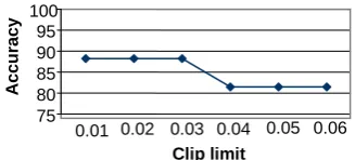
The Figure 3 shows the effect of clip limit on accuracy, used in CLAHE as discussed in section 3. The value of the clip limit is varied from 0.01 to 0.05 and is observed that from 0.01 to 0.03 the accuracy is stable (88.24), from 0.04 the accuracy drops (81.65).
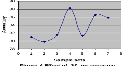
Figure 4 shows the classification accuracy for eight data sets of benign and malign classes with different dimensions. The sets of different dimensions are obtained, by keeping the size of one class fixed and by varying the size of the other class and then vice versa. The accuracy starts increasing as the difference in sample size decreases, reaches a peak at a certain point, where difference is small and then starts to decrease.
The choice of sigma in the Eq 5 has a fair impact on the classification accuracy. The sigma value is varied from 0.1 to 1, and the results are shown in Figure 5 in terms of accuracy. It is clear that the proposed system achieves best classification rate at 0.6, then there is deterioration in accuracy.
The number of features used for classification, also has great impact on classification accuracy. The variance in classification accuracy for different number of features is illustrated in Figure 6. The number of features used is experimented from 5 to 35. The accuracy of the classifier increases as number of features increases reaches a peak and then begins to decrease. The classifier gives its best accuracy for a total of 20 features.
5.
CONCLUSION
In this paper, multi-transform based properties of normal, benign and malign ROI are investigated with KDA in
classifying mammograms. Through the experiments it is found that the classifier works excellently for finite sample sizes and the classification rate varies as the dimensions of sample sizes changes, hence experiments are done to improve the classification rate with variant sample sizes. The study reveals that, the dimensions of complementary classes, number of features used as well as the band width parameter controls the classifier’s performance. All the three tuning parameters are dependent on nature of dataset used and there exists no direct formula to find them, hence the values are found through cross validation. In future the performance of KDA classifier will be analyzed by assigning weights to misclassified samples.
6.
REFERENCES
[1] Sheila Timp, Celia Varela, and Nico Karssemeijer, ‘Computer-Aided Diagnosis With Temporal Analysis to Improve Radiologists Interpretation of Mammographic Mass Lesions’, IEEE transactions on information technology in biomedicine, VOL. 00, NO. 00, 2010
[2] Mohamed Meselhy Eltoukhy , Ibrahima Faye , Brahim Belhaouari Samir . ‘Breast cancer diagnosis in digital mammogram using multiscale curvelet Transform’. Computerized Medical Imaging and Graphics 34 (2010) 269–276
[3] Essam A Rashed, Ismail A Ismail and Sherif I. Zaki. ‘ Multiresolution mammogram analysis in multilevel decomposition ’. Pattern Recognition Letters, 28, 2007, pp 286–292.
[4] Hao Jing, Yongyi Yang, Laura M. Yarusso and Robert M. Nishikawa, ‘Textural feature comparison between FFDM and Film mammograms’, IEEE conference on Biomedical Imaging, 2011.
[5] Meigui Chen, Qingxiang Wu, Rongtai Cai,Chengmei Ruan and Lijuan Fan, ‘Extraction of breast cancer areas in mammography using neural network based on multiple features’, Proceedings of third international conference on Artificial Intelligence and computational intelligence, Vol. 3, ISBN: 978-3-642-23895-6, 2011
[6] Shantanu Banik, Rangaraj M. Rangayyan, and J. E. Leo Desautels, ‘Detection of Architectural Distortion in Prior Mammograms’, IEEE Transactions on Medical Imaging, Vol.30,No.2, pp.279-294, 2011
[7] Peter Mc Leod and Brijesh Sharma, “Variable Hidden Neuron Ensemble for Mass Classification in Digital Mammograms”, IEEE ComputatIonal Intelligence magazine February 2013, PP.no. 68-76
[8] Zhimin Huo, Maryellen L. Giger, and Carl J. Vyborny, “Computerized Analysis of Multiple-Mammographic Views: Potential Usefulness of Special View Mammograms in Computer-Aided Diagnosis ”, IEEE Transactions on Medical Imaging, VOL. 20, NO. 12, December 2001 pp.no1285-1292
[9] Arianna Mencattini, Marcello Salmeri, Giulia Rabottino and Simona Salicone, “Metrological Characterization of a CADx System for the Classification of Breast Masses in Mammograms ”, IEEE Transactions on Instrumentation and Measurement, VOL. 59, NO. 11, November 2010, pp no. 2792-2799
[image:5.595.78.242.190.264.2][10]http://peipa.essex.ac.uk/ipa/pix/mias/(publicly available mammogram database)
Figure 6 Effect of number of features
30 25 20 15 10
5 35
65 70 75 80 85 90 95 100
Number of features
A
c
c
u
ra
c
y
Figure 3 Effect of clip limit on accuray
0.06 0.05 0.04 0.03 0.02 0.01 75 80 85 90 95 100
Clip limit
A
c
c
ura
c
y
[image:5.595.61.263.506.597.2][11]Ahmed, N. Natarajan, T. ; Rao, K.R., “ Discrete Cosine Transform ”, IEEE Transactions on Computers, Vol.C-23 , ,Issue: 1 Jan. 1974 PP no.90 - 93
[12]S Mallat. “A theory for multiresolution signal decomposition: The wavelet representation", IEEE Transaction Pattern Analysis Machine Intelligence. Vol 11, no 7, Jul. 1989, pp 674–693.
[13]Comparative Study of Techniques for Large-Scale Feature Selection. F.J. Ferria, P. Pudilb, M. Hatefc and J. Kittlerc a Dept. Inform atica i Electr onica. Universitat ..
[14]Marco Di Marzio, Charles C.Taylor. ‘Kernel Density Classification and Boosting ’.citeseer ,biometrica,vol 91,pp. 226-223