Reliability of river control structures

information.

Author(s):Marriott, Martin John; Andrews, I.G. Title:Reliability of river control structures Year of publication:2007

Citation:Marriott, M.J., Andrews, I.G. (2007) ‘Reliability of river control structures' Proceedings of Advances in Computing and Technology, (AC&T) The School of Computing and Technology 2nd Annual Conference, University of East London, pp.184-191

Link to published version:

RELIABILITY OF RIVER CONTROL STRUCTURES

M.J.Marriott*, I.G.Andrews**

**Environment Agency [email protected]

Abstract: This paper concerns reliability centred management of river control structures. Reliability concepts are reviewed, and presented in a straightforward single parameter format appropriate for use in this context. A case study is presented that illustrates the described approach, and investigates the connection between reliability and maintenance expenditure. Correlation was found between lower reliability and both total and preventative maintenance expenditure, but little correlation with the amount of reactive maintenance expenditure.

1. Introduction

Reliability is commonly understood as a measure of the dependability of an asset, and is an important consideration within the general challenge of asset management. Asset management is an increasingly important activity that may be defined as a system or process to manage equipment to maximise its lifetime value. This involves not only achieving a balance between different forms of maintenance strategies (such as reactive and preventative), but also includes emergency and contingency planning, audits and performance reviews, life cycle cost analysis and analysis of causes of failure.

For the management of flood control structures, where each asset must be ready to perform as designed when required, a successful asset management strategy should be reliability centred. Unless flood control structures are appropriately managed over their lifetime, the full benefit of the initial capital investment may not be realised. This paper presents a framework for analysing reliability data that may be applied in the context of river structures, which are usually

unique installations with relatively little operational data when compared with the mass produced objects to which reliability theory is often applied in the manufacturing industry. The resulting information may be useful in a decision support model for helping to focus maintenance activity on flood defence structures.

2. Flood risk management context

It is preferable to speak of flood risk management, rather than control or defence, to avoid giving a false sense of security. Recent trends in flood risk management have been to recognise formally the benefits of reducing the impact of flooding through improved flood forecasting and warning, and development control, as well as reducing the probability of flooding by traditional construction methods, including reliance on control structures, which need to operate reliably.

methods to the performance and reliability of flood and coastal defences. Those methods produce fragility curves as a plot of probability of failure against hydraulic loading for a flood alleviation system, but the present paper deals with the reliability of a particular component, namely river control structures, for which the reliability is not generally dependent upon the hydraulic loading.

3. Reliability theory

Reliability of an item may be defined as the probability that the item performs a required function for a given time. Alternatively this may be stated as the probability of no failure occurring over a given time interval.

To make use of data about times to failure in order to predict reliabilities, it is necessary to select and fit an appropriate probability distribution. Many different probability distributions may be used, but a popular general purpose distribution in manufacturing contexts is the Weibull distribution, with three parameters (scale, shape and location) in its most general form.

3.1. The Weibull distribution

The three parameters in the general form of the Weibull distribution are given many different symbols in different texts, but using α, β and γ respectively, for the scale, shape and location parameters, the probability density function (pdf), f(t), may be written:

( )

f (1)

The so called location parameter γ is in effect a lower limit which all times to failure

zero to give a two parameter analysis. A number of civil engineering examples of such applications are given by Metcalfe (1997). Kankam (2002) applied a two parameter analysis in his study of water supply pipelines, and Hames (2006) also uses this approach for the threshold method of analysis of extreme sea water levels. Failure rates often follow a classic pattern widely known as the bathtub curve, with three distinct regions corresponding to early failure, followed by a useful life with an approximately constant failure rate, and ending in a wear out period where the failure rate increases with time. Bentley (1993), in a text relating particularly to electrical, mechanical and manufacturing engineering, considered it adequate for a large range of products and components to concentrate on the useful life period and therefore to employ a constant failure rate model (sometimes referred to as a constant instantaneous failure rate, or hazard rate). The possible increased initial failure rate could be considered to be removed by ‘burn in’ techniques for electrical components or other commissioning procedures during a contractual defects liability period. Arguably for long life control structures there is not an imminent risk of wear out. Therefore the constant failure rate model seems appropriate in this context, as well as being suited to the data available. For this constant failure rate approach, the shape parameter β in equation (1) is set to unity, and that leaves only the scale parameter α to be determined. This may be shown to equal the mean life time of the component, in this case. The inverse of this parameter is the failure rate (λ), and applying these simplifications to equation (1) yields the following pdf:

( )

This equation (2) is in fact the one parameter version of the Exponential distribution. It applies in the region t≥0, producing a skewed distribution that is clearly preferable for this purpose to the normal or Gaussian distribution, which would in theory include impossible negative values of t.

The pdf from equation (2) may be integrated to give the cumulative distribution function (cdf), F(t):

( )

( )

0 e 1 dt t f t

F =

_∫

and reliability R(t) is the complement of this:

( )

( )

R = − = −λ (4)

The mean time to failure (MTTF) is given by

( )

= −λ ∞

∞

∫

MTTF

0 t

0

(5)

which is the result stated above for the mean life time of a component. For repairable items, the mean time between failures (MTBF) is employed.

3.2. The Poisson distribution

An alternative derivation comes from the link with the well known Poisson distribution that may be used to model random discrete events. Consider the number of failures occurring in a time t and having a Poisson distribution with mean value λt, then:

( ) ( )

P x t

λ −

λ

= (6)

where x = 0,1,2 …, and λ is a constant which represents the failure rate.

So the reliability is equal to the probability of no occurrences in time t, given by:

( ) ( )

R = = −λ (7)

which is the same result as given in equation (4) above.

In this formulation the parameter λ represents failure rate (e.g. failures per year) and its inverse gives the mean time to fail, or in cases where components are repaired rather than replaced, the mean time between failures (MTBF e.g. in years). The MTBF is equivalent to the scale factor α in the one parameter version of the Weibull distribution:

λ = 1

MTBF (8)

This may be used to fit the probability distribution to failure data. For example, if 3 failures are recorded in 6 years, and downtime is considered negligible, then the MTBF is 2 years, and the estimated failure rate λ is 0.5 failures per year. This value of λ may then be used in equation (7) to estimate reliability over a selected time period t.

4. Application

As explained above, available performance data may be used in equation (8) to estimate λ. This value may in turn be used to calculate a reliability figure from equation (7). In the study in question this was expressed as a percentage probability of meeting a year long operational commitment without any unplanned outages.

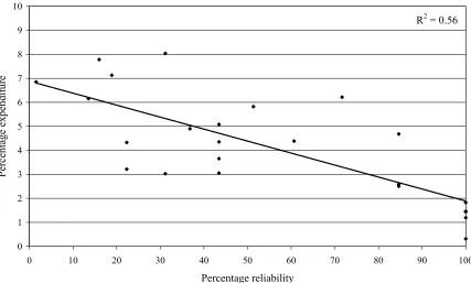
incident that resulted in the structure failing to perform as designed, and that would result in an increased flood risk. So an electrical power failure would only be classified as a failure if the structure was not self operating and was dependent on power to operate a gate. For the purposes of this paper the intended or designed method of operation was considered in isolation from any backup or contingency arrangements that were in place. The reason for this approach was to focus on the designed method of operation rather than to test contingency arrangements which may include back up generation or alternatives such as manual hand wound operation. The data was drawn from 24 river control structures over a 6 year period. The types of structure have been listed in Table 1. The aim is to illustrate the method of analysis, and to draw conclusions regarding maintenance expenditure and reliability in general. An initial plot on Figure 1 shows total maintenance expenditure against reliability of the structure. A trend is evident from structures with low reliability (frequent failure) and higher maintenance expenditure, to those with high reliability and lower maintenance expenditure.

About three quarters of the total maintenance is classified as preventative, and this is shown in Figure 2 plotted against reliability, with a similar pattern to total maintenance. This indicates that the structures which required significant preventative maintenance were also likely to be less reliable.

The remaining maintenance is unplanned work mainly in reaction to an operational failure, and this is shown in Figure 3. There is surprisingly little correlation here between reactive maintenance expenditure and lower reliability. An explanation may be that the

necessarily expensive to fix.

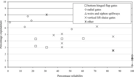
The trend lines shown on Figures 1 to 3 are least squares straight line fits to the data, with the R2 values as calculated in Microsoft Excel shown in the top right hand corner of each figure. Figure 4 shows the same total maintenance expenditure as Figure 1, but divided into the different categories of structure, and without the trend line. Figure 4 shows a range of performance from radial gates generally to the top left of the graph with higher maintenance requirements and lower reliability, to the passive structures (fixed weirs and siphons) which do not rely on automated movement of gates, at the bottom right of the graph as might be expected. It would be hard to draw firm conclusions about the merits of the different automated active control structures from this data, with considerable overlap in performance. However, the approach to determining a quantitative reliability figure enables the data to be presented in a way that enables such a comparison to be made, given sufficient data. The importance of gathering such data is emphasised, for the benefit of future design and for management of maintenance of such assets.

5. Conclusions

Firstly, the one parameter exponential distribution is shown to be a simplified version of the Weibull distribution, as well as a result from assuming that failure follows a Poisson process. These approaches are common in reliability analysis, and it is useful to appreciate the links between them.

Thirdly, the results from the case study indicate the obvious point that passive structures (weirs, siphons) are more reliable than active structures. There also appears to be a trend connecting lower reliability with higher amounts of preventative maintenance. However, perhaps surprisingly, there appears to be little correlation connecting lower reliability with higher amounts of reactive maintenance expenditure.

Finally, it is noted that references for this paper draw on work in civil engineering, pipeline technology, electrical, mechanical and manufacturing engineering, and the first author would be keen to discuss and collaborate with colleagues with similar interests, with a view to publication of a broader study of methods used in practice to quantify reliability.

6. Acknowledgements:

This paper draws on data initially analysed by the second author under the supervision of the first author whilst at the University of Hertfordshire (Andrews, 2001); this has been subsequently revisited and the analysis extended. The authors are grateful to the Environment Agency for permission to use the data and publish this paper, and wish to emphasise that conclusions presented are their personal views and not necessarily those of their employers.

7. References:

Andrews I.A., Flood Control Structures

Asset Management, MSc Project Report,

University of Hertfordshire, 2001.

Bentley J.P., An Introduction to Reliability

and Quality Engineering. Longman

Scientific & Technical, 1993

Hames D.P., Personal communication regarding coastal engineering teaching material for the MSc Civil Engineering at University of East London, 2006

Kankam K.K. Study of service life of PVC-U

pressure pipes, MPhil Dissertation,

University of East London, 2002.

Metcalfe A.V., Statistics in Civil

Engineering, Arnold 1997

Sayers P.B., Hall J.W. and Meadowcroft I.C., “Towards risk-based flood hazard management in the UK”, Proceedings of the Institution of Civil Engineers, Civil

Engineering, 150, May 2002, 36-42

Simm J.D. and Camilleri A.J., “Construction risk in coastal and river engineering”,

Journal of the Chartered Institution of

Water and Environmental Management, 15,

Reliability Data Maintenance Expenditure as % of Overall Total

Type of Structure

Interval (yr)

Number of failures

MTBF (yr)

One year Reliability

(%)

Preventative Reactive Total

Bottom hinged flap gate

6 9 0.67 22 3.0 1.3 4.3

Bottom hinged flap gate

6 7 0.86 31 2.6 0.4 3.0

Bottom hinged flap gate

6 3 2.00 61 2.6 1.8 4.4

Bottom hinged flap gate

6 5 1.20 43 2.8 1.5 4.4

Bottom hinged flap gate

4 6 0.67 22 2.6 0.7 3.2

Radial gate 6 10 0.60 19 5.3 1.9 7.1

Radial gate 6 12 0.50 14 5.2 0.9 6.2

Radial gate 6 11 0.55 16 4.7 3.1 7.8

Radial gate 6 25 0.24 2 5.6 1.2 6.9

Radial gate 6 4 1.50 51 4.9 0.9 5.8

Vertical lift sluice gate

6 5 1.20 43 3.0 0.6 3.7

Vertical lift sluice gate

6 2 3.00 72 4.2 2.0 6.2

Vertical lift sluice

gate 6 1 6.00 85 1.6 1.0 2.6

Vertical lift sluice

gate 6 1 6.00 85 1.6 0.9 2.5

Vertical lift sluice gate

6 1 6.00 85 4.0 0.7 4.7

Vertical lift sluice gate

6 5 1.20 43 3.9 1.2 5.1

Vertical lift sluice gate

6 6 1.00 37 4.5 0.4 4.9

Vertical lift sluice gate

6 5 1.20 43 1.7 1.4 3.1

Labyrinth weir 6 0 - 100 0.9 0.3 1.2

Fixed weir 6 0 - 100 1.2 0.3 1.5

Labyrinth weir 6 0 - 100 1.0 0.4 1.4

Siphon spillway 6 0 - 100 0.3 0.0 0.3

Siphon spillway 6 0 - 100 1.7 0.1 1.8

Automatic Pointer gate

6 7 0.86 31 6.7 1.3 8.0

R2 = 0.56

0 1 2 3 4 5 6 7 8 9 10

0 10 20 30 40 50 60 70 80 90 100

Percentage reliability

Percentage

expe

ndit

ur

e

Figure 1: Total maintenance expenditure versus reliability

R2 = 0.53

0 1 2 3 4 5 6 7 8 9 10

0 10 20 30 40 50 60 70 80 90 100

Percentage reliability

Per

cen

tage

expe

ndit

ur

e

R2 = 0.17

0 1 2 3 4 5 6 7 8 9

0 10 20 30 40 50 60 70 80 90 100

Percentage reliability

Perc

entage expenditure

Figure 3: Reactive maintenance expenditure versus reliability

0 1 2 3 4 5 6 7 8 9 10

0 10 20 30 40 50 60 70 80 90 100

Percentage reliability

P

er

centa

ge ex

pend

itur

e

bottom hinged flap gates radial gates

weirs and siphon spillways vertical lift sluice gates other