Combining deep and handcrafted image features for MRI brain scan classification

Combining deep and handcrafted image 

features for MRI brain scan classification

Hasan, A, Jalab, HA, Meziane, F, Kahtan, H and Al­Ahmad, AS

http://dx.doi.org/10.1109/ACCESS.2019.2922691

Title

Combining deep and handcrafted image features for MRI brain scan 

classification

Authors

Hasan, A, Jalab, HA, Meziane, F, Kahtan, H and Al­Ahmad, AS

Type

Article

URL

This version is available at: http://usir.salford.ac.uk/id/eprint/51567/

Published Date

2019

USIR is a digital collection of the research output of the University of Salford. Where copyright 

permits, full text material held in the repository is made freely available online and can be read, 

downloaded and copied for non­commercial private study or research purposes. Please check the 

manuscript for any further copyright restrictions.

Combining Deep and Handcrafted Image Features

for MRI Brain Scan Classification

ALI M. HASAN1_{, HAMID A. JALAB} 2_{, (Member, IEEE), FARID MEZIANE} 3_,

HASAN KAHTAN4, (Member, IEEE), AND AHMAD SALAH AL-AHMAD 5 1_{College of Medicine, Al-Nahrain University, Baghdad 10072, Iraq}

2_{Faculty of Computer Science and Information Technology, University of Malaya, Kuala Lumpur 50603, Malaysia} 3_{School of Science, Engineering, and Environment, University of Salford, Salford M5 4WT U.K.}

4_{Faculty of Computer Systems and Software Engineering, Universiti Malaysia Pahang, Pahang 26600, Malaysia} 5_{College of Business Administration, American University of the Middle East, Al-Ahmadi 54200, Kuwait}

Corresponding author: Hamid A. Jalab (hamidjalab@um.edu.my)

This work was supported by the research and innovation of university Malaysia Pahang under Fundamental Research Grant Scheme (FRGS) No: RDU190189.

ABSTRACT Progresses in the areas of artificial intelligence, machine learning, and medical imaging technologies have allowed the development of the medical image processing field with some astonishing results in the last two decades. These innovations enabled the clinicians to view the human body in high-resolution or three-dimensional cross-sectional slices, which resulted in an increase in the accuracy of the diagnosis and the examination of patients in a non-invasive manner. The fundamental step for magnetic resonance imaging (MRI) brain scans classifiers is their ability to extract meaningful features. As a result, many works have proposed different methods for features extraction to classify the abnormal growths in the brain MRI scans. More recently, the application of deep learning algorithms to medical imaging leads to impressive performance enhancements in classifying and diagnosing complicated pathologies, such as brain tumors. In this paper, a deep learning feature extraction algorithm is proposed to extract the relevant features from MRI brain scans. In parallel, handcrafted features are extracted using the modified gray level co-occurrence matrix (MGLCM) method. Subsequently, the extracted relevant features are combined with handcrafted features to improve the classification process of MRI brain scans with support vector machine (SVM) used as the classifier. The obtained results proved that the combination of the deep learning approach and the handcrafted features extracted by MGLCM improves the accuracy of classification of the SVM classifier up to 99.30%.

INDEX TERMS Deep learning, MGLCM, MRI brain scans, feature extraction, SVM classifier.

I. INTRODUCTION

Medical imaging is the practice of acquiring diagnostic images by using a range of technologies to produce accurate representation of patients’ body for the purposes of diagnosis, monitoring or treatment of medical conditions. It is consid-ered as a one of the most powerful available resources to gain a direct insight of the human body with no needs for surgery or other invasive procedures. Each type of medical imaging technology provides different information about the pathological area being studied or treated [1]. Recently image processing has been embedded in most medical systems, which deal with the information used by clinicians to ana-lyze and diagnose any pathological area in a short-time. The

The associate editor coordinating the review of this manuscript and approving it for publication was Md. Asikuzzaman.

importance of image processing includes the improvement of pictorial information for clinicians and processing of these information for an autonomous machine perception [2].

Brain tumors are abnormal and uncontrolled propagation of cells inside the brain which are categorized into two major groups; primary tumors which originate in the brain tissue itself and secondary tumors which spread from somewhere else in the body to the brain through the blood stream [3]. The choice of treatment can vary depending on the tumor location, type and size. In most cases, surgery is considered as the treatment of choice for brain tumors that can be reached without any risks and side effects to the brain [4].

Medical imaging is one type among many technologies that are utilized to view the internal organs of the human body through cross-sectional slices to diagnose, and monitor the medical conditions. These technologies give different

A. M. Hasanet al.: Combining Deep and Handcrafted Image Features for MRI Brain Scan Classification

information about the pathological area being stud-ied or treated [3]. Among these medical technologies is magnetic resonance imaging (MRI) which is a volumetric imaging modality that gives information about the posi-tion, and size of the tumors. MRI technology is based on observing the behavior of protons’ orientation inside a large magnetic field after manipulating radiofrequency wave and recovering their equilibrium state [5]. The provided scans by MRI scanners include a very high diagnostic value which can be used to diagnose and monitor some physiological processes such as water diffusion and blood oxygenation. MRI is competent to precisely differentiate soft tissues with high resolution and is more sensitive to tissue density changes that reflect the physiological alternation. The spatial res-olution is a process of digitizing the collected signal by MRI scanner and allocating a value to each pixel in the original image. Currently, the voxel size of 1×1×1 mm is achievable [6], [7].

An MRI session may last from 30 minutes to an hour depending on the human body area being scanned and the number of MRI slices that are collected; the number of slices being influenced by the scanner’s resolution and the slice thickness. In a clinical routine, these MRI slices are evaluated, diagnosed and interpreted by clinicians, which increases their workloads leading to an increased allocated work time [2].

The advantages of MRI technology comprise non-ionizing radiation, high resolution imaging, superior soft tissue con-trast resolution and different pulse sequences. Moreover, the output of an MRI investigation is a set of images for tissue with different contrast visualization. These pulse sequences provide valuable anatomical information that help clinicians diagnose the pathological conditions precisely [8]. The MRI technologies are categorized into: T1-weighted (T1-w) images which are routinely used in neuroimaging studies. They are used as an anatomical reference, because they are characterized by a high resolution and less artifacts. For instance, a black hole in the brain looks as a hypo-intense or dark area relative to the white matter (WM) inten-sities. On the other hand, T2-weighted (T2-w) images are an important MRI sequences that are suitable for recognizing the boundaries of pathological structures, where most of these structures produce hyper-intense signals due to high water content, while much less common of these pathological struc-tures appear as a hypo-intense or dark area in T2-weighted images [9]. The main drawback of T2-weighted sequence is that the intensity distributions of cerebrospinal fluid (CSF), grey matter (GM) and tumors are closed together. Clinically, the use of these two MRI sequences are essential in diag-nosing brain tumors but can produce some difficulties in dif-ferentiating tumors from non- tumorous areas in addition to grading [10]. Subsequently, a utilization of contrast medium is important to clarify the tumor boundary compared with non- tumorous tissue on T1-w and T2-w images.

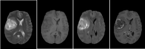
Some types of brain tumors are complicated because they are not enhanced with contrast medium usage. Therefore, fluid attenuated inversion recovery (FLAIR) protocol with

FIGURE 1. Samples of four abnormal(pathological) MRI slices, from left to right T2-w, T1-w, FLAIR and T1c-w.

T2-w scan is used to show the non-enhanced brain tumors [10], [11]. Fig. 1 shows four samples of T2-w, T1-w, T1-w with contrast enhancement (T1c-w) and FLAIR images.

The aim of any diagnostic imaging technique is the char-acterization of regions in images that are measured by texture analysis. Texture analysis is considered to be an efficient way to quantify intuitive qualities by measuring the spatial variation in pixel intensities [12]. Moreover, texture analysis is a potentially indispensable tool in neuro-MR imaging, such that the anatomical structures of the brain in MR images can be characterized by texture analysis better than the human visual examination [13].

The classification process of MRI brain scans involves two components; image feature extraction and image classifica-tion. Since the feature extraction process plays a significant role in image classification, a diversity of feature extraction algorithms have been proposed to extract MR image features. However, not all of these methods are adaptive to different MR image classification problems.

Following the success of convolutional neural networks as an alternative approach for automatical feature extrac-tion method from images while training [14], we propose a new feature extraction method based on convolutional neural networks (CNN) which allow us to extract a wide range of features, then combined these features with handcrafted features that are extracted by using the modified grey level co-occurrence matrix (MGLCM) method for classification of MRI brain scans which represent the main contribution of this study.

For the CNN based deep learning feature extraction, a sim-ple CNN architecture is used. One input layer is used, fol-lowed by three convolutional layers and two pooling layers, and ended by a fully connected layer.

The rest of the paper is organized as follows: Section 2 reviews some related state-of-art methods that have been proposed recently; Section 3 provides the details of the proposed method of MRI brain tumors classification; Section 4 presents the experimental results and finally, the conclusions are given in Section 5.

II. RELATED WORK

Texture analysis has been studied for a long period and researchers have developed different methods for automated brain tumor classification. Hasan and Meziane [2] applied a new modified gray level co-occurrence matrix (MGLCM)

to extract statistical texture features which were enough to discriminate the normality and abnormality of the brain by using a single MRI modality (T2-w). A classification accu-racy of 97.4% was achieved by using a multi-layer perceptron neural network (MLP) classifier.

Nabizadeh and Kubat [15] used five efficacious statis-tical texture extraction methods: first order statisstatis-tical fea-tures, gray level run length matrix (GLRLM), local binary pattern (LBP), gray level co-occurrence matrix (GLCM), and histogram of oriented gradient (HOG). The achieved classification accuracy to classify a database that included 25 abnormal (pathological) MRI brain scan was 97.40% Sachdeva et al. [16] used GLCM, Laplacian of Gaussian (LoG), Gabor wavelet, rotation invariant local binary pat-terns (RILBP), intensity-based features (IBF) and shape-based features (SBF) to develop an automated system to classify MRI brain tumors. The features were optimized by using a genetic algorithm (GA). Both MLP, and SVM were used individually to classify brain tumors in MRI scans and the achieved accuracies were 91.7% and 94.9%, respectively.

Recently, the use convolutional neural networks (CNNs) in multiple medical imaging disciplines started outperforming other proposed models in medical image classification. CNNs represent powerful tools for extracting features and learning useful characteristic or attribute of medical images. Many of the handcrafted features of image that are extracted by traditional methods and fed to classification methods are typically ignored compared to complex features which are learnt automatically by CNNs [17], [18] Chen et al. [19] used several convolutions and pooling layers to extract the deep features from hyperspectral image (HSI). Experimen-tally, the best results were achieved by using three layers of CNN with convolution kernel size of 4×4 or 5×5 and a pooling kernel in each layer of 2×2 van der Burghet al.[20] applied a deep learning algorithm to predict the remaining time of amyotrophic lateral scleral sick person using both the MRI scan, and the clinical characteristics, such that, the clinical characteristics and MRI data are combined into a layered CNN which further improved the predictions about the survival time. Deepening artificial neural networks bring machine learning closer to artificial intelligence. The use of deep learning can enable the extraction of new features that have never been discovered previously [21] Wicht [22], used deep learning networks to extract automatically rele-vant features from images in an unsupervised manner and compared these features against handcrafted features. The author concluded that learned features by deep learning were superior to handcrafted features. Moreover, the deep learning approach is more adaptable to work on a variety of datasets.

Automatic brain tumor classification is a very challenging task in large spatial and structural variability of surrounding region of brain tumor. The use of deep learning was also applied for classification of tumor regions in MRI images. An automatic classification method for brain tumor using CNN approach was proposed by [5]. The accuracy achieved

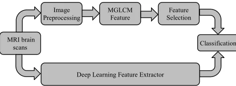
FIGURE 2. Flow chart of the proposed algorithm.

was 97.5% with low complexity. A new tumor classification approach using CNN was proposed by [23]. The experimental results of the classification accuracy of cranial MR images is 97.18%. Another approach for MRI classification was pro-posed by [24] in which a dataset of 66 brain MRI were used to classify tumors into 4 classes (i.e. normal, glioblastoma, sarcoma and metastatic bronchogenic carcinoma tumors). The experimental results achieved 96.97% classification accuracy. In the handcrafted methods of feature extraction, regardless of which features are extracted, it is not adequate to extract all important features of the medical images. As a result, we need to perform a combination between hand craft and deep learning as a new feature extraction approach to improve the classification task.

III. PROPOSED METHOD

The aim of this study is to improve the accuracy of MRI brain scans classification by combining handcrafted (MGLCM) and deep learning (DF) features. The process of this study is shown in Fig. 2. It starts with the dataset that was collected and classified into normal and abnormal (pathological) MRI scans.

The proposed method comprises the following stages: MRI scan preprocessing, the MGLCM feature extrac-tion, deep learning feature extracextrac-tion, and finally the classification.

A. MRI SCAN PREPROCESSING

A. M. Hasanet al.: Combining Deep and Handcrafted Image Features for MRI Brain Scan Classification

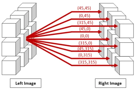
FIGURE 3. The relationship between the reference pixels and the opposite nine pixels.

B. THE MGLCM FEATURE EXTRACTION

MGLCM is a statistical method which was modified by Hasan and Meziane [2], and was used to extract the second-order texture features by inspecting the combined frequencies of all grey levels of pixel configuration of each pixel in the left hemisphere (reference pixel) with one of nine opposite pixels that exist in the right hemisphere. These features measure statistically the degree of symmetry between both sides of the brain. Symmetry is an important parameter that is used within the diagnosing process to detect the normality and abnor-mality of the human brain. Consequently, nine co-occurrence matrices are extracted for each MRI slice under nine offsets

θ=(45,45), (0,45), (315,45), (45,0), (0,0), (315,0), (45,315), (0,315), (315,315), and one distance as shown in Fig. 3. The co-occurrence relative frequencies between joint pixels are calculated after normalization by the total sum of all its elements, equation (1) [2]:

P(i,j)_(θ1,β2)= 1

2562

M

X

x=1

N

X

y=1

×

  

 

1, ifL(x,y)=_i

andR(x+1x,y+1y)=j

0, otherwise

(1) where L and R are the left and right parts of the brain’s hemispheres respectively,M andN are the width and height of MRI slice respectively, i and j are the co-occurrence matrix’s coordinates, 1x and 1y values are subject to the directions of measured matrix and undergo to a set of rules that are demonstrated clearly in [2], and P is the resulting co-occurrence matrix.

There are twenty-one texture measures extracted from each co-occurrence matrix and these measures represent the most common and widely-used texture features [28]. Hasan and Meziane [2] refined these texture measures by ignoring the irrelevant features using analysis of variance method (ANOVA) and reduced to eleven texture measures for each co-occurrence matrix, namely, the contrast, the dissimilarity, the correlation, the sum of square variance, the sum variance,

FIGURE 4. Convolution of a 5×5 image with a 3×3 kernel.

the sum average, the difference entropy, the inverse difference normalized (IDN), the information measure of correlation I (IMC1), the inverse difference moment normalized (IDMN) and the weighted distance in addition to the cross correlation. The total number of texture measures was reduced from 190 to 100 feature measures after using ANOVA.

C. DEEP LEARNING FEATURE EXTRACTION

Deep neural networks, or more concretely, the convolutional neural networks (CNNs) are an adaptation of the artificial neural network. The multiple layers of convolutions with pooling layers are used as a mapping function to transform a multidimensional MRI slice into a desired output after training [17]. The advantage of applying deep learning is that the network learns to extract features while training. Deep neural networks or CNNs extract features by themselves using their convolution kernels. Additionally, there is a set of small parameterized filters in the convolutional layers. They are usually called kernels or convolutional filters, and are applied to every layer to produce a tensor of feature maps as shown in Fig. 4. How far the filter moves in every step from one position to the next position is named ‘a stride’. In practice, only strides by one and two pixels perform well, while increasing the stride more declines the performance of CNNs significantly [20]. Moreover, the stride must be set in a way that the output volume is an integer and not a fraction. In some cases, if the convolution filter does not cover all the input image, zero-padding is needed to pad the border of input image with zeros to keep always the same spatial dimensions. The feature maps that are produced from a convolutional layer, are calculated through rectified linear unit (ReLU) activation function in the activation layer. The ReLU is the most commonly used activation function in deep learning models that is used to suppress all negative values in the feature maps to zero [17]. The rectified feature maps are fed through the pooling layers to reduce the dimensionality by generating small non-overlapped regions as input and deter-mine a single value for each region. Two popular functions are the max function and the average function, which are frequently used in the pooling layer [17], [20], [21]. A batch normalization layer is typically used after activation layers to normalize feature maps. This layer works as a regulator

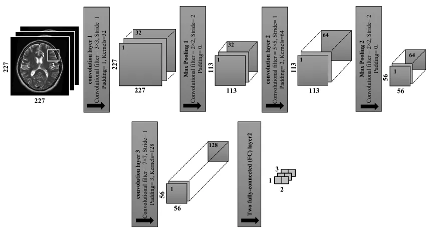
FIGURE 5. Architecture of deep CNN as features extractor with three convolutional layers and two pooling layers.

for the network, and speeds up the training process [21]. The last convolutional layer is followed by the fully-connected layer (FC).

The power of CNN depends essentially on how the network is architected and how the layers are connected as well as how the proper weights are set. Gradient back-propagation represents the main algorithm for learning all types of neural networks [19], [20].

To design a new CNN architecture of CNN for a specific task, it is essential to understand the requirements to be met and how the data is fed to the network. The size of each convolutional layer for a given MRI slice can be determined by using equation (2) and equation (3) respectively:

Convwidth =

MRISlicewidt−Cfwidth+(2×ZP)

Swidth

+1 (2)

Convheight =

MRISliceheight−Cfheight+(2×ZP)

Sheight

+1

(3) whereCf denotes the convolutional filter,ZPis the number of zero padding if required, andSrefers to the number of strides. The architecture of the CNN network with input images of 227 ×227 pixels is illustrated in the following steps and shown in Fig. 5:

i- Conv1(convolutional filters of size 3×3, stride of 1,

padding of 1, and kernels of 32) are applied.

Conv1=

227−3+(2×1)

1 +1=227 For the square feature maps, there are 227×227×

32= 1648928 neurons in the feature map of the first convolution layer.

ii- MaxPooling₁ is equal to the previous image size divided by the stride number:

Max Pooling1=

227 2 ≈113

For the square feature maps, there are 113×113×32=

408608 neurons in the feature map of the first max pooling layer.

iii- Conv2(convolutional filters of size 5×5, stride of 1,

padding of 2 and kernels of 64) are applied.

Conv2=

113−5+(2×2)

1 +1=113 For the square feature maps, there are 113×113 ×

64=817216 neurons in the feature map of the second convolution layer.

iv- MaxPooling₂ is determined by the same way that is used inMaxPooling₂:

Max Pooling2=

113 2 ≈56

For the square feature maps, there are 56×56×64=

200704 neurons in the feature map of the second max pooling layer.

v- Conv3(convolutional filters of 7×7 applied with stride

of 1, padding of 3 and kernels of 128).

Conv3=

56−7+(2×3)

1 +1=56

For the square feature maps, there are 56×56×128

= 401408 neurons in the feature map of the third convolution.

A. M. Hasanet al.: Combining Deep and Handcrafted Image Features for MRI Brain Scan Classification

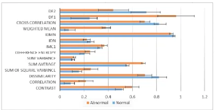
FIGURE 6. Extracted features (mean±standard deviation) of normal and pathological MRI brain scans.

layers. The output size of FC is equal to the number of classes of the data set. In this study the input size of FC is equal to 401408 and the output size is equal to 2. In the proposed algorithm, the mean and standard deviation between the two groups (normal, and abnormal) are calcu-lated for MGLCM features and for deep feature (DF) extrac-tion process. As shown in Fig. 6 the combined features that are extracted by the proposed method, significantly reflect the changes between the normal and pathological MRI brain scans.

IV. EXPERIMENTAL RESULTS

In this study, a total of 6000 MRI axial slices from 600 patients (300 normal, and 300 abnormal) were collected from the Iraqi center for research and magnetic resonance of Al-Kadhimain Medical City. These MRI scans were acquired using SIMENS MAGNETOM Avanto 1.5 Tesla scanner and PHILIPS Achieva 1. 5 Tesla, that have plane resolutions (256 ×256) and (512×512) respectively. The voxel res-olution of the latter is (1 ×1×3 mm3) and the former is (1×1×5mm3). The number of slices for each MRI scan is about 75 slices. The collected dataset was diagnosed and classified into normal and pathological scan by the clinicians of this center. T2-w images are used in this study due to their high sensitivity to tissue pathology and clearly show tumor boundaries. The collected MRI dataset is adopted to validate the proposed method. Support vector machine (SVM) with 10-fold cross validation method are applied for accuracy rate estimation of the proposed method. The dataset is divided randomly into 10 folds that are roughly of equal size. Each MRI slice in the given dataset was normalized with ‘zero-center’ before submission to CNN. A sample of the images dataset is shown in Fig. 7. The first row is for normal class images, while the second row is for abnormal class images. The code was developed using MATLAB 2018b (The Math-Works Inc., USA).

The architecture design of CNN was optimized by using a trial and error approach which was used to determine the optimal number of convolutional layers, number of neurons in each layer, learning rate and kernel size.

Table 1 summarizes the architecture of the CNN which is used in this study. There are seven layers, ordered as I, C1, C2,

FIGURE 7. Sample of used images dataset.

TABLE 1.Architecture of CNN as feature extractor.

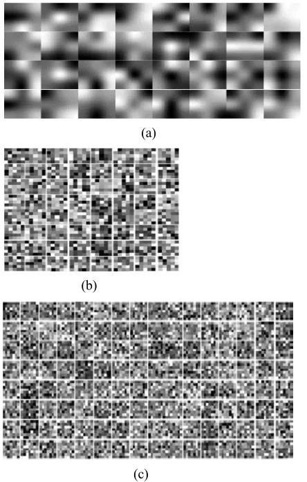
C3, P4, P5 and F6 in sequence. Where, I is the input layer, C represents the convolutional layers, P represents the pooling layers and F refers to the fully connected layer. Weights play a pivotal role in CNN. Fig. 8 shows the weights of a convolutional kernels of the three convolutional layers of CNN.

In the training process of deep learning, the momentums are set to 0.9. The initial learning rate is 0.0001, and the max iteration number is 100. The training process graph is shown in Fig. 9. By looking at the result shown in Fig. 9, we could see that the training accuracy shows an increasing trend with respect to the number of iterations. This indicates the good performance of the proposed CNN architecture for the classification process of MRI brain scans.

It is noted that different features may be extracted using different convolution kernels and they become more and more abstract after using several convolutional and pooling layers. In this study, the effectiveness of deep learning features is evaluated and compared with the MGLCM features through classification results using the quadratic SVM. The image dataset is randomly divided into 10 folds with equal size. Nine folds for training, while the remainder is used for testing. The MATLAB R2018b (MathWorks, Natick, MA, USA) on Windows 10 is used to implement the proposed method.

In the proposed algorithm, the mean and standard devia-tion measures can numerically summarize the experimental results. These measures are calculated for MGLCM features and for deep feature (DF) extraction process. As shown in Fig. 10, the mean and standard deviation give a clue about statistical significance between normal and abnormal groups of features extracted by the MGLCM and DF.

FIGURE 8. Learned weights of the convolutional layers of CNN, (a) learned weights of first convolutional layer (1×32), (b) learned weights of second convolutional layer (1×64), and (c) learned weights of third convolutional layer (1×128).

FIGURE 9. The training process of deep learning.

The performance is also evaluated by calculating the TN which symbolizes the number of true negatives (abnormal) cases, and TP which means the number of true positives (normal) cases.

The performances of two methods MGLCM and DF of fea-ture extraction and the proposed MGLCM-DF are presented in Table 2.

A classification accuracy rate of 99.30% is obtained by the proposed method MGLCM-DF. The next best performance is

FIGURE 10. The average means standard deviations for extracted features of normal and abnormal (pathological) MRI scan by DF and MGLCM feature extractions.

TABLE 2.The performances of two methods MGLCM, DF, and proposed MGLCM-DF.

FIGURE 11. The ROC curve of the MGLCM-DF feature extraction.

achieved by deep learning features (97.80%). The MGLCM texture features method produced an accuracy rate of 96.10%. Moreover, the proposed MGLCM-DF is capable of combin-ing the advantages of hand-crafted MGLCM texture features and deep learned features DF to improve the classification accuracy rate by the SVM classifier.

The ROC curve for the classification results of the pro-posed MGLCM-DF is shown in Fig. 11. The ROC curve was evaluated by considering the normal cases in MRI images as a positive class (TP), and the abnormal cases in MRI images as a negative class (FP). We can see that the normal cases accuracy is (1.00) which represents 100% accuracy for the normal cases. The area under curve (AUC) is 1.00, showing the best classification accuracy for using MGLCM-DF.

A. M. Hasanet al.: Combining Deep and Handcrafted Image Features for MRI Brain Scan Classification

TABLE 3. The performances of proposed DF and other pre-trained deep learning networks using same collected image dataset.

TABLE 4. Comparison with other methods.

through using three standard pre-trained deep learning net-works (AlexNet, GoogleNet, and SqueezeNet) and the results are presented in Table 3. AlexNet is a CNN of 8 layers deep and used to classify images into 1000 classes. GoogLeNet is a pre-trained model 144 layers, and can classify images into 1000 classes. And finally, the SqueezeNet is a pre-trained model, and can classify images into 1000 classes. The code was developed in MATLAB 2018b (The MathWorks Table.

Using the transfer learning through using existing pre-trained models forced feature extraction and classification processes to follow the same pre-trained module which is not similar to the problem we want to solve.

In this study we developed our model for feature extraction by using both MGLCM and deep learning (DF) and combin-ing them in one feature set which is considered as the main contributions of this study [29].

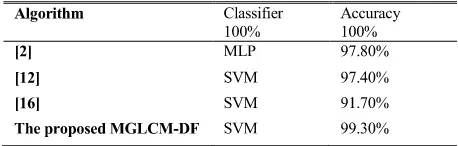
The comparison of the proposed MGLCM-DF with other three works using standard BRATS 2013 MRI dataset is shown in Table 4. The proposed MGLCM-DF method obtained the highest accuracy rate, while the classification methods in [2], [12], [16] achieved accuracy rates of 97.80%, 97.40%, and 91.70%, respectively. The high accuracy rate by the proposed MGLCM-DF proves the appropriate combina-tion of the feature extraccombina-tion which makes the classificacombina-tion error significantly lower.

V. CONCLUSION

This study proposes a new method (MGLCM-DF) to improve the classification process of MRI brain scans. It comprises a modified texture features extraction (MGLCM) method, combined with deep learning features (DF). In the proposed MGLCM-DF, the MGLCM hand-craft texture features and the deep learning features are extracted from MRI brain scans, then combined as one final feature to improve the classification process of MRI brain scans. The MGLCM-DF was capable of combining the benefits of MGLCM and DF

as a new approach for feature extractions for improving the classification process of MRI brain scans. The experimental results of MGLCM-DF show a classification accuracy rate of 99.30% when performed on the collected dataset of MRI brain scans. The proposed method can be improved in future studies as a reliable brain tumor feature extraction for classi-fication method to be used with different medical images.

ACKNOWLEDGMENT

The authors would like to thank the anonymous reviewers for their valuable suggestions and comments to improve this manuscript.

REFERENCES

[1] R. W. Ibrahim, A. M. Hasan, and H. A. Jalab, ‘‘A new deformable model based on fractional wright energy function for tumor segmentation of vol-umetric brain MRI scans,’’Comput. Methods Programs Biomed., vol. 163, pp. 21–28, Sep. 2018.

[2] A. M. Hasan and F. Meziane, ‘‘Automated screening of MRI brain scanning using grey level statistics,’’Comput. Elect. Eng., vol. 53, pp. 276–291, Jul. 2016.

[3] G. S. Tandel, M. Biswas, O. G. Kakde, A. Tiwari, H. S. Suri, M. Turk, J. R. Laird, C. K. Asare, A. A. Ankrah, N. N. Khanna, B. K. Madhusudhan, L. Saba, and J. S. Suri, ‘‘A review on a deep learning perspective in brain cancer classification,’’Cancers, vol. 11, no. 1, p. 111, 2019.

[4] American Brain Tumor Association, Chicago, IL, USA. (2015).Surgery. [Online]. Available: http://www.abta.org/secure/surgery.pdf

[5] S. Pereira, A. Pinto, V. Alves, and C. A. Silva, ‘‘Brain tumor segmentation using convolutional neural networks in MRI images,’’IEEE Trans. Med. Imag., vol. 35, no. 5, pp. 1240–1251, May 2016.

[6] A. M. Hasan, F. Meziane, and M. A. Kadhim, ‘‘Automated segmentation of tumours in MRI brain scans,’’ presented at the 9th Int. Joint Conf. Biomed. Eng. Syst. Technol. (BIOSTEC), Rome, Italy, 2016. [Online]. Available: http://www.scitepress.org/DigitalLibrary/PublicationsDetail. aspx?ID=obG7gAh7vJI=&t=1

[7] G. Vishnuvarthanan, M. P. Rajasekaran, P. Subbaraj, and A. Vishnuvarthanan, ‘‘An unsupervised learning method with a clustering approach for tumor identification and tissue segmentation in magnetic resonance brain images,’’ Appl. Soft Comput., vol. 38, pp. 190–212, Jan. 2016.

[8] R. Gurusamy and V. Subramaniam, ‘‘A machine learning approach for MRI brain tumor classification,’’Comput., Mater. Continua, vol. 53, no. 2, pp. 91–108, 2017.

[9] A. Zimny, M. Neska-Matuszewska, J. Bladowska, and M. J. Sa¸siadek, ‘‘Intracranial lesions with low signal intensity on T2-weighted MR images–review of pathologies,’’Polish J. Radiol., vol. 80, p. 40, Jan. 2015. [10] N. B. Bahadure, A. K. Ray, and H. P. Thethi, ‘‘Image analysis for MRI based brain tumor detection and feature extraction using biologically inspired BWT and SVM,’’Int. J. Biomed. Imag., vol. 2017, Mar. 2017, Art. no. 9749108.

[11] H. A. Jalab and A. Hasan, ‘‘Magnetic resonance imaging segmentation techniques of brain tumors: A review,’’Arch. Neurosci., vol. 6, Jan. 2019, Art. no. e84920. doi:10.5812/ans.84920.

[12] N. Nabizadeh, ‘‘Automated brain lesion detection and segmentation using magnetic resonance images,’’ Ph.D. dissertation, Dept. Elect. Comput. Eng., Univ. Miami, Coral Gables, FL, USA, 2015.

[13] S. Tantisatirapong, ‘‘Texture analysis of multimodal magnetic resonance images in support of diagnostic classification of childhood brain tumours,’’ Ph.D. dissertation, School Electron., Elect. Comput. Eng., Univ. Birming-ham, BirmingBirming-ham, U.K., 2015.

[14] X. Yang and Y. Fan, ‘‘Feature extraction using convolutional neural net-works for multi-atlas based image segmentation,’’Proc. SPIE, vol. 10574, Mar. 2018, Art. no. 1057439.

[15] N. Nabizadeh and M. Kubat, ‘‘Brain tumors detection and segmentation in MR images: Gabor wavelet vs. Statistical features,’’J. Comput. Elect. Eng., vol. 45, pp. 286–301, Jul. 2015.

[16] J. Sachdeva, V. Kumar, I. Gupta, N. Khandelwal, and C. K. Ahuja, ‘‘A package-SFERCB-‘segmentation, feature extraction, reduction and classification analysis by both SVM and ANN for brain tumors,’’’Appl. Soft Comput., vol. 47, pp. 151–167, Oct. 2016.

[17] A. S. Lundervold and A. Lundervold, ‘‘An overview of deep learning in medical imaging focusing on MRI,’’Zeitschrift für Medizinische Physik, vol. 29, no. 2, pp. 102–127, 2019.

[18] A. Işın, C. Direkoğlu, and M. Şah, ‘‘Review of MRI-based brain tumor image segmentation using deep learning methods,’’Procedia Comput. Sci., vol. 102, no. 2016, pp. 317–324, 2016. doi:10.1016/j.procs.2016.09.407.

[19] Y. Chen, H. Jiang, C. Li, X. Jia, and P. Ghamisi, ‘‘Deep feature extrac-tion and classificaextrac-tion of hyperspectral images based on convoluextrac-tional neural networks,’’IEEE Trans. Geosci. Remote Sens., vol. 54, no. 10, pp. 6232–6251, Oct. 2016.

[20] H. K. van der Burgh, R. Schmidt, H.-J. Westeneng, M. A. de Reus, L. H. van den Berg, and M. P. van den Heuvel, ‘‘Deep learning predictions of survival based on MRI in amyotrophic lateral sclerosis,’’NeuroImage, Clin., vol. 13, pp. 361–369, Oct. 2017. doi:10.1016/j.nicl.2016.10.008.

[21] J. Liu, Y. Pan, M. Li, Z. Chen, L. Tang, C. Lu, and J. Wang, ‘‘Applications of deep learning to MRI images: A survey,’’Big Data Mining Anal., vol. 1, no. 1, pp. 1–18, Mar. 2018.

[22] B. Wicht, ‘‘Deep learning feature extraction for image processing,’’ Ph.D. dissertation, Dept. Inform., Univ. Fribourg, Fribourg, Switzerland, 2017.

[23] A. Ari and D. Hanbay, ‘‘Deep learning based brain tumor classification and detection system,’’Turkish J. Elect. Eng. Comput. Sci., vol. 26, no. 5, pp. 2275–2286, 2018.

[24] H. Mohsen, E.-S. A. El-Dahshan, E.-S. M. El-Horbaty, and A.-B. M. Salem, ‘‘Classification using deep learning neural networks for brain tumors,’’Future Comput. Informat. J., vol. 3, no. 1, pp. 68–71, 2018. [25] A. M. Hasan, F. Meziane, R. Aspin, and H. A. Jalab, ‘‘MRI brain scan classification using novel 3-D statistical features,’’ inProc. 2nd Int. Conf. Internet Things Cloud Comput., 2017, Art. no. 138.

[26] A. M. Hasan, F. Meziane, R. Aspin, and H. A. Jalab, ‘‘Segmentation of brain tumors in MRI images using three-dimensional active contour without edge,’’Symmetry, vol. 8, no. 11, pp. 132, 2016.

[27] A. M. Hasan, ‘‘A hybrid approach of using particle swarm optimization and volumetric active contour without edge for segmenting brain tumors in MRI scan,’’Indonesian J. Elect. Eng. Inform., vol. 6, no. 3, pp. 292–300, 2018.

[28] K. Lloyd, P. L. Rosin, D. Marshall, and S. C. Moore, ‘‘Detecting violent and abnormal crowd activity using temporal analysis of grey level co-occurrence matrix (GLCM)-based texture measures,’’Mach. Vis. Appl., vol. 28, nos. 3–4, pp. 361–371, 2017.

[29] B. H. Menze et al. ‘‘The multimodal brain tumor image segmenta-tion benchmark (BRATS),’’IEEE Trans. Med. Imag., vol. 34, no. 10, pp. 1993–2024, Oct. 2015.

ALI M. HASAN received the B.Sc. and M.Sc. degrees from the University of Technology, Iraq, in 2002 and 2004, respectively, and the Ph.D. degree from the University of Salford, U.K., in 2017. Since 2005, he has been a Lecturer with Al-Nahrain University, Iraq. His research interest includes image processing and segmentation.

HAMID A. JALABreceived the B.S. degree in electrical engineering from the University of Tech-nology, Iraq, and the M.Sc. and Ph.D. degrees in computer systems from Odessa National Polytech-nic University. He is currently an Associate Pro-fessor with the Faculty of Computer Science and Information Technology, University of Malaya, Malaysia. He has authored more than 100 indexed papers and ten national research projects. His research interests include digital image processing and computer vision.

FARID MEZIANE received the Ph.D. degree in computer science from the University of Salford, where he is involved in producing formal speci-fication from natural language requirements. He is currently the Chair of Data and Knowledge Engineering and the Director of the Informatics Research Centre with the University of Salford, U.K. He has authored over 100 scientific papers and participated in many national and international research projects. His research interests include natural language processing, semantic computing, data mining, and big data and knowledge engineering. He is also the Co-Chair of the International Conference on the Application of Natural Language to Information Systems and in the programme committee of over ten international conferences and in the editorial board of three international journals. He was awarded the Highly Commended Award from the Literati Club, 2001 for his paper on Intelligent Systems in Manufacturing: Current Development and Future Prospects.

HASAN KAHTANreceived the B.Sc. degree from the University of Baghdad, and the M.Sc. and Ph.D. degrees in computer science from Univer-siti Teknologi Mara, Malaysia, in the field of software engineering and software security. He is currently a Senior Lecturer with the Faculty of Computer Systems and Software Engineering, Universiti Malaysia Pahang. His research inter-ests include software engineering, software secu-rity and dependability attributes, and machine learning.