SOMANI’S Approximation Method(SAM) Innovative Method for finding optimal Transportation Cost

© 2015, IRJET.NET- All Rights Reserved Page 493

SOMANI’S Approximation Method(SAM)

Innovative Method for finding optimal Transportation Cost

CHIRAG SOMANI*

Asst. Prof. in Mathematics

Department of Applied Science & Humanities, Engineering College, Tuwa, Godhra, Gujarat Pin Code- 388713

Gujarat Technological University, Ahmadabad

Abstract

Transportation problem is one of the sub classes of Linear Programming Problem(LPP) in which the objective is to transport various quantities of a single product that are stored at various origins to several destinations in such a way that the total transportation cost is minimum. The costs of shipping from sources to destinations are indicated by the entries in the matrix. To achieve this objective we must know the amount and location of available supplies and the quantities demanded. The different solution procedure of such type of problem illustrate in given paper.

Keywords: Transportation problem, source, destination, SAM Method.

Introduction:

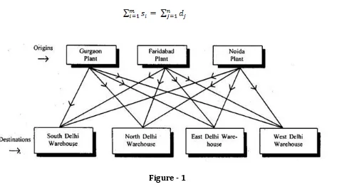
The Transportation problem is one if the original application of Linear Programming Problem. The main objective of transportation problem is to minimize the cost of transportation from the source to destination while satisfying supply as well as demand. Two contributions are mainly responsible for such type of problem which involves a number of sources and the number of destinations. Transportation problems may involve movement of a product from plants to warehouses, warehouses to wholesalers, wholesalers to retailers and retailers to customers. This problem can be used for a variety of situations such as scheduling, inventory control, personnel assignment, plant location etc.

Basic Hypothesis in Transportation Problem:

(1)Total Quantity of the item available at a different source equally the total demand at different destination.

(2)Product can be transported easily from all sources to destinations.

(3)The unit transportation cost of the item from all sources to destinations is known.

(4)The transportation cost on a given route is directly proportion to the number of units shipped on that route.

© 2015, IRJET.NET- All Rights Reserved Page 494

Mathematical Representation of Transportation Problem:

The Transportation problem can be formulated into a LP problem. Let xij , i = 1 ….m, j = 1 …n be the

number of units transported from origin i to destination j. The LP problem is as follows –

Minimize:

Subject to: ( i = 1, 2, - - -, m)

( j = 1, 2, - - -, n)

( i = 1, 2, - - -, m, j = 1, 2, - - - n).

A transportation problem is said to be balanced if

Figure - 1

SAM Method:

© 2015, IRJET.NET- All Rights Reserved Page 495

Step -1 Make transportation table for given problem and convert into balance one if it is not.

Step -2 Finding minimum element of each row.

Step -3 Compare the minimum element of each row and put the demand according the supply on which element that the mathematical value is minimum.

Step -4 If the row demand and supply is equal then next step we will find the remaining rows minimum element and follow step -3 whenever the demand and supply are not satisfy.

Step -5 Incase demand and supply are not equal then we again find the minimum element of each rows and follow step -3.

Step -6 If the minimum element are same then we can firstly allocate those minimum element which demand is minimum.

Step -7 now same process follows whenever all given supply and demand not satisfy.

Step -8 after satisfying demands and supply of each column and row multiply Allocated row or column element with allocation values.

Step -9 add all this multiplied value this is the required transportation cost is given Problem.

Some Problems:

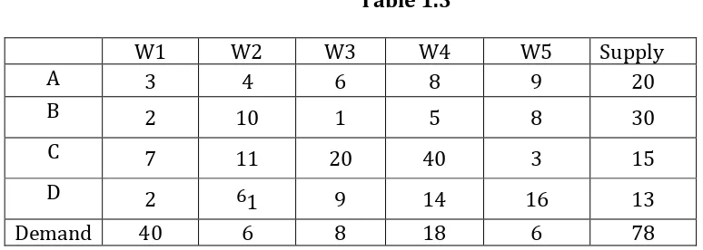
Problem-1 Solve the given transportation problem-

Table 1.1

W1 W2 W3 W4 W5 Supply

A 3 4 6 8 9 20

B 2 10 1 5 8 30

C 7 11 20 40 3 15

D 2 1 9 14 16 13

Demand 40 6 8 18 6 78

Solution - Step- 1 Supply and demand of Product is equal so the problem is balanced.

© 2015, IRJET.NET- All Rights Reserved Page 496 Table 1.2

A 3

B 1

C 3

D 1

Step -3 Compare the minimum element of each row and put the demand according

the supply on which element that the mathematical value is minimum. So the minimum value is B=1 and D=1. Allocation s made on D because the demand of D is minimum to B.

Table 1.3

W1 W2 W3 W4 W5 Supply

A 3 4 6 8 9 20

B _{2 10 1 5 8 30}

C _{7 11 20 40 3 15}

D ₂ 6_{1 9 14 16 13}

Demand 40 6 8 18 6 78

Step- 4 The demand of W2 is over. Now again find the minimum value of each row

excluding W2.

Table 1.4

A 3

B 1

C 3

D 2

Minimum Value is B=1. Now allocation is made on B=1.

Table 1.5

W1 W2 W3 W4 W5 Supply

A _{3 4 6 8 9 20}

B _{2 10} 8_{1 5 8 30}

© 2015, IRJET.NET- All Rights Reserved Page 497

D ₂ 6_{1 9 14 16 13}

Demand 40 6 8 18 6 78

Step -5 same process follow whenever all demand and supply are not satisfy. In case

the minimum element is same then we can firstly allocate those minimum elements which demand is minimum.

The demand of W3 is over. Now again find the minimum value of each row excluding W2 & W3.

Table 1.6

A 3

B 2

C 3

D 2

Minimum Value is B=2 and D=2. So first we will allocate D=2

Table 1.7

W1 W2 W3 W4 W5 Supply

A _{3 4 6 8 9 20}

B _{2 10} 8_{1 5 8 30}

C _{7 11 20 40 3 15}

D 7₂ 6_{1 9 14 16 13}

Demand 40 6 8 18 6 78

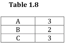
The demand of W1 is not over. But supply of D is over. Now again find the minimum value of each row excluding W2, W3 & D.

Table 1.8

A 3

B 2

C 3

Minimum Value is B=2. Now allocation is made on B=2.

© 2015, IRJET.NET- All Rights Reserved Page 498

W1 W2 W3 W4 W5 Supply

A 3 4 6 8 9 20

B 22_{2 10} 8_{1 5 8 30}

C _{7 11 20 40 3 15}

D 7₂ 6_{1 9 14 16 13}

Demand 40 6 8 18 6 78

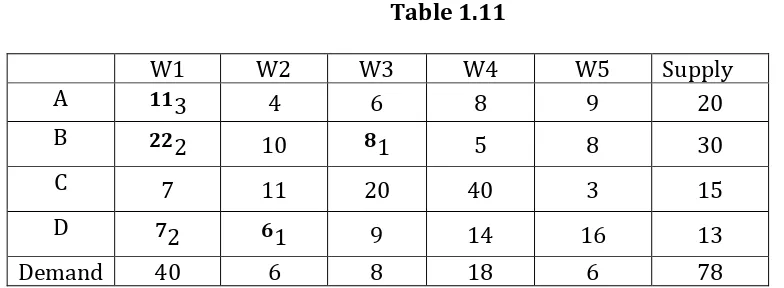
The demand of W1 is not over. But supply of B is over. Now again find the minimum value of each row excluding W2, W3, D & B.

Table 1.10

A 3

C 3

Minimum Value is A=C=3. Now allocation is made on A=3 because its demand is minimum to C.

Table 1.11

W1 W2 W3 W4 W5 Supply

A 11_{3 4 6 8 9 20}

B 22_{2 10} 8_{1 5 8 30}

C _{7 11 20 40 3 15}

D 7₂ 6_{1 9 14 16 13}

Demand 40 6 8 18 6 78

The demand of W1 is over. Now again find the minimum value of each row excluding W1, W2, W3, D & B.

Table 1.12

A 8

C 3

Minimum Value is C=3. Now allocation is made on C=3.

© 2015, IRJET.NET- All Rights Reserved Page 499

W1 W2 W3 W4 W5 Supply

A 11_{3 4 6 8 9 20}

B 22_{2 10} 8_{1 5 8 30}

C _{7 11 20 40} 6_{3 15}

D 7₂ 6_{1 9 14 16 13}

Demand 40 6 8 18 6 78

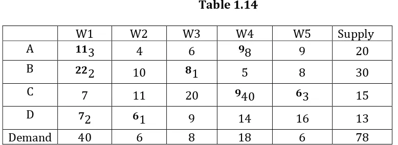
The demand of W5 is over. The last column W4 is remaining. Put the demand according to supply of each row.

Table 1.14

W1 W2 W3 W4 W5 Supply

A 11_{3 4 6} 9_{8 9 20}

B 22_{2 10} 8_{1 5 8 30}

C _{7 11 20} 9₄₀ 6_{3 15}

D 7₂ 6_{1 9 14 16 13}

Demand 40 6 8 18 6 78

Step -6 After completion of all allocation the allocated element multiplied by same row element.

Mini Transportation Cost

= 11*3 + 9*8 + 22*2 + 8*1 + 9 *40 + 6*3 + 7*2 + 6*1 = 555 Rs.

Therefore the solution of problem is A11 = 11, A14 = 9, B11 = 22, B13 = 8, C14 = 9 C15 = 6, D11

= 7, D12 = 6 and the transportation cost is = 555 Rs.

Conclusion:

© 2015, IRJET.NET- All Rights Reserved Page 500

Reference:

1. Sultan, A. & Goyal, S.K. (1988). Resolution of Degeneracy in Transportation Problems, J Opl Res Soc 39, 411-413.

2. en.wikipedia.org/wiki/operations_research

3. Sharma J K. Quantitative Techniques (2007). (6th ed.). New Delhi: Macmillan. 4. Munkres, J. (1957). “Algorithms for the Assignment and Transportation

5. Problems”, Journal of the Society for Industrial and Applied Mathematics, 5(1),32-38. 6. www.phpsimplex.com/en/history/htm

7. www.charlesbabbage.net

8. T.C. Koopman (1947): “Optimum utilization of transportation system”, Proc. Intern. Statics. Conf. Washington D.C.

9. Khurana, A. and Arora, S. R. (2011). Solving Transshipment Problem with mixed constraints. International journal of Management Science and Engineering Management. 6(4):292-297.

10.Ji Ping & Chu, K. F. (2002). A dual matrix approach to the transportation problem. Asia-Pacific Journal of Operations Research, 19, 35-45.

11.Goyal S. K. (1984). Improving VAM for the Unbalance Transportation Problem, J Opl Res Soc 35, 1113-1114.

12.Dantzig, G. B.; Fulkerson, R.; Johnson, S. M. (1954), "Solution of a large-scale traveling salesman problem", Operations Research 2 (4): 393–410, doi:10.1287/opre.2.4.393, JSTOR 166695.

13.Adlakha, V., Kowalski, K. & Lev, B. (2006). Solving Transportation Problem with Mixed Constraints, JMSEM 1, 47-52.

14.E. E. Ammar and E. A. Youness (2005): “Study on multi-objective transportation problem with fuzzy numbers”, Applied Mathematics and Computation, 166: 241-253