doi:10.5194/hess-16-1047-2012
© Author(s) 2012. CC Attribution 3.0 License.
Earth System
Sciences
Global patterns of change in discharge regimes for 2100
F. C. Sperna Weiland1,2, L. P. H. van Beek1, J. C. J. Kwadijk2, and M. F. P. Bierkens1,3
1Department of Physical Geography, Utrecht University, P.O. Box 80115, 3508 TC Utrecht, The Netherlands 2Deltares, P.O. Box 177, 2600 MH Delft, The Netherlands
3Deltares, P.O. Box 80015, 3508 TA Utrecht, The Netherlands
Correspondence to: F. C. Sperna Weiland ([email protected])
Received: 9 November 2011 – Published in Hydrol. Earth Syst. Sci. Discuss.: 13 December 2011 Revised: 3 March 2012 – Accepted: 22 March 2012 – Published: 2 April 2012
Abstract. This study makes a thorough global assessment of the effects of climate change on hydrological regimes and their accompanying uncertainties. Meteorological data from twelve GCMs (SRES scenarios A1B and control experiment 20C3M) are used to drive the global hydrological model PCR-GLOBWB. This reveals in which regions of the world changes in hydrology can be detected that have a high like-lihood and are consistent amongst the ensemble of GCMs. New compared to existing studies is: (1) the comparison of spatial patterns of regime changes and (2) the quantifica-tion of notable consistent changes calculated relative to the GCM specific natural variability. The resulting consistency maps indicate in which regions the likelihood of hydrological change is large.
Projections of different GCMs diverge widely. This un-derscores the need of using a multi-model ensemble. De-spite discrepancies amongst models, consistent results are revealed: by 2100 the GCMs project consistent decreases in discharge for southern Europe, southern Australia, parts of Africa and southwestern South-America. Discharge de-creases strongly for most African rivers, the Murray and the Danube while discharge of monsoon influenced rivers slightly increases. In the Arctic regions river discharge in-creases and a phase-shift towards earlier peaks is observed. Results are comparable to previous global studies, with a few exceptions. Globally we calculated an ensemble mean discharge increase of more than ten percent. This increase contradicts previously estimated decreases, which is amongst others caused by the use of smaller GCM ensembles and dif-ferent reference periods.
1 Introduction
Climate change will have notable effects on global runoff regimes and will affect water availability for agriculture and ecosystems as well (Arnell, 2003; Liu et al., 2008, 2009; Oki and Kanae, 2006; V¨or¨osmarty et al., 2000). To antic-ipate for these changes, reliable assessments of the hydro-logical effects of climate change, including information on uncertainties are needed (Murphy et al., 2004; Giorgi and Mearns, 2002; IPCC, 2007). Studies investigating hydrolog-ical effects of climate change on continental or global scale are often based on results from General Circulation Models (GCMs). However, especially for precipitation, GCMs pro-duce quite varying and even contradictory results (Covey et al., 2003; Meehl et al., 2000).
al., 2011) is required. Such extensive assessments will in the end provide important information on local water availabil-ity, conditions for navigation, ecosystems and hydropower generation.
Table A, provided as Supplement, provides an overview of previous hydrological impact assessments which are dis-cussed in this study. All these studies focus on change in runoff or discharge, Table A (in the Supplement) lists the dif-ferences in various aspects. This comparison provides some background information for this current study and enables us to evaluate the value of the different techniques used in hy-drological impact assessments.
Overall the results of these studies project a decrease in runoff for southern Europe, north and south Africa, south-western USA, Mexico and Brazil and an increase in dis-charge for Monsoon driven and Arctic rivers. Several studies (Alcamo and Henrichs, 2002; Arnell, 1999, 2003; Nijssen et al., 2001; V¨or¨osmarty et al., 2000) used a change fac-tor method instead of directly applying the climate model data for the future period. Within the change factor method observed precipitation, temperature or runoff fields are ad-justed with a change factor derived from climate model data and those adjusted time-series are then used to derive fu-ture runoff and discharge changes. The method assumes that change is more reliable than absolute values. However, this only holds under the assumption of a constant model bias through time. Furthermore change in variability is ignored (Fowler et al., 2007). Although computationally more de-manding than the change factor method, directly forcing a hydrological model with climate model data for current and future climate and calculation of differences in obtained dis-charges may give more reliable estimates of changes in vari-ability and extremes.
Change in runoff can also directly be derived from runoff fields calculated by GCMs (Sperna Weiland et al., 2011). Unfortunately such data is not accessible for most models and in most GCMs river routing is not included. To obtain information on changes in river regimes, additional routing of GCM runoff fields is needed (Arora and Boer, 2001; Milly et al., 2005; Nohara et al., 2006). To this end river discharge is most often calculated with a hydrological model that in-cludes a routing model, using either meteorological variables directly from GCMs (Aerts et al., 2006) or using observed meteorological time series perturbed with change factors de-rived from GCM results (Alcamo and Henrichs, 2002; Ni-jssen et al., 2001; V¨or¨osmarty et al., 2000).
For a climate effect study it is possible to select datasets from multiple GCMs for multiple emission scenarios. Ar-nell (2003) showed that by 2050 there is little difference be-tween the emission scenarios, i.e. correspondence bebe-tween GCMs is weaker than between scenarios. This indicates that the choice of GCMs highly influences the calculated change and it has been concluded before that a multi-model en-semble of GCMs provides the most reliable impression of the spread and uncertainties of possible changes (Boorman
and Sefton, 1997; IPCC, 2007; Murphy et al., 2004). Ar-nell (2003), Milly et al. (2005), Nohara et al. (2006) and Ni-jssen et al. (2001) used these multi-model ensembles.
All studies in Table A (see Supplement) indicated direc-tions and amount of change for world regions or river basins, however quantification of the significance of these changes frequently played a minor role. In this study we will make a thorough assessment of the global hydrological effects of climate change by directly applying daily climate data from an ensemble of twelve GCMs for the IPCC SRES scenario A1B for the period 2081–2100 as input to the global hydro-logical model PCR-GLOBWB. In this hydrohydro-logical model river discharge is calculated using an explicit routing scheme based on the kinematic wave equation, which also includes temporal storage in flood plains, lakes, wetlands and reser-voirs. The relative changes between the current and future climate are analyzed instead of absolute changes, hereby re-ducing the influence of biases in the hydrological model and GCM data.
In addition, to investigating annual mean changes in runoff fields and changes in river regimes as has also been done in previous studies, we will here focus on: (1) spatial pat-terns of change in the annual cycle looking at changes in timing of peak, (2) additional discharge statistics (e.g. maxi-mum and minimaxi-mum flow and interannual discharge variabil-ity), (3) likelihood of change which is calculated here for each model individually relative to its inter-annual variabil-ity, and finally focus will be on (4) the consistency amongst model projections on the direction of change. This enables us to indicate on world maps in which regions the likelihood of hydrological changes is large.
2 Methods
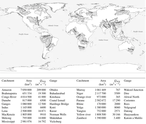
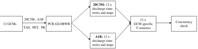
The distributed global hydrological model PCR-GLOBWB (Van Beek et al., 2011; Van Beek and Bierkens, 2009; Bierkens and van Beek, 2009) was run on a daily time-step with meteorological time series from 12 GCMs for the 20C3M experiment for the period 1971–1990 and the SRES scenarios A1B for the period 2081–2100. From the results we derived change fields of discharge regimes for which the consistency amongst GCMs was quantified. We selected 19 large catchments (Fig. 1) which cover a variety of cli-mate zones, latitudes and continents. For these catchments changes in the mean annual cycle are quantified. The setup of the study is schematized in Fig. 2.
2.1 Hydrological model
F. C. Sperna Weiland et al.: Global patterns of change in discharge regimes for 2100 1049
Fig. 1. Selected catchments with total catchment area, average observed discharge (Qavg; GRDC, 2007) and location of gauges for which
statistics are calculated, annual cycles are given and comparisons are made.
Catchment Area Qavg Gauge Catchment Area Qavg Gauge
(km2) (m3s−1) (km2) (m3s−1)
Amazon 7 050 000 209 000 Obidos Murray 1 061 469 767 Wakool Junction
Brahmaputra 651 334 19 300 Bahadurabad Niger 2 117 700 5589 Dire
Congo River 4 014 500 41 000 Kinshasa Orange river 973 000 365 Aliwal North
Danube 817 000 6500 Ceatal Izmail Parana 2 582 672 17 290 Corientes
Ganges 1 080 000 12 500 Hardinge Bridge Rhine 170 000 2000 Rees
Indus 1 165 000 6600 Kotri Volga 1 380 000 8060 Volgograd
Lena 2 500 000 16 871 Kusur Yangtze 752 000 2571 Datong
MacKenzie 1 805 000 9910 Norman Wells Yellow river 1 808 500 30 166 Huayuankou
Mekong 795 000 16 000 Mukdahan Zambezi 1 390 000 3.400 Katom a Mulilo
Mississippi 2 981 076 16 792 Vicksburg
a realistic annual river discharge cycle (Sperna Weiland et al., 2011). Here only a short description of the model is provided, for an extended description and evaluation of the model see Van Beek et al. (2011).
Each PCR-GLOBWB model cell consists of two vertical soil layers and one underlying groundwater reservoir. Sub-grid parameterization is used to represent fractions of short and tall vegetation, surface water and for calculation of satu-rated areas to quantify surface runoff and lateral outflow from the unsaturated zone. Water enters the cell as rainfall and can be stored as canopy interception or snow. Snow accumula-tion or melt depends on temperature (degree day method) and melt water and throughfall are passed to the surface. Evapo-transpiration is calculated from the potential evaporation and soil moisture conditions. Vertical exchange of water is
possi-ble between the soil and groundwater layers. Runoff is made up of non-infiltrating melt and throughfall water, saturation excess surface runoff, interflow and base flow. For each time-step the water balance is computed per cell. Runoff is ac-cumulated and routed as river discharge along the drainage network taken from DDM30 (D¨oll and Lehner, 2002) using the kinematic wave approximation of the Saint-Venant equa-tion. Adaptations have been made to the network to improve the inclusion of storage in lakes, wetlands and large reser-voirs. Hereto a selection of substantial lakes and reservoirs (≥500 km2) was obtained from the GLWD1 data set (Lehner and D¨oll, 2004). The resulting river discharge represents nat-ural flow. Water and reservoir management, river regulation and other human influences have not been included. Model parameterization is based on best available global datasets
www.hydrol-earth-syst-sci.net/16/1/2012/ Hydrol. Earth Syst. Sci., 16, 1–16, 2012
Fig. 1. Selected catchments with total catchment area, average observed discharge (Qavg; GRDC, 2007) and location of gauges for which statistics are calculated, annual cycles are given and comparisons are made.
a realistic annual river discharge cycle (Sperna Weiland et al., 2011). Here only a short description of the model is provided, for an extended description and evaluation of the model see Van Beek et al. (2011).
Each PCR-GLOBWB model cell consists of two vertical soil layers and one underlying groundwater reservoir. Sub-grid parameterization is used to represent fractions of short and tall vegetation, surface water and for calculation of sat-urated areas to quantify surface runoff and lateral outflow from the unsaturated zone. Water enters the cell as rainfall and can be stored as canopy interception or snow. Snow accumulation or melt depends on temperature (degree day method) and melt water and throughfall are passed to the surface. Evapotranspiration is calculated from the potential evaporation and soil moisture conditions. Vertical exchange
12 GCMs PCR-GLOBWB
12 x GCM specific
T-statistics 20C3M , A1B
TAS, PET, PR
20C3M:12 x discharge time-series and maps
A1B:12 x discharge time-series and maps
[image:4.595.106.497.63.160.2]Concistency check
Fig. 2. Schematization of experimental setup.
available global datasets and so far the model has not been calibrated. More information about the model performance can be found in Van Beek et al. (2011).
Because of some apparent deviations, mostly caused by biases in meteorological forcing and additionally by sim-plifications in model structure and related scale issues, we will focus on relative changes between current and future discharges instead of absolute values. To overcome initial-ization problems, initial states have been obtained for each GCM dataset individually. For the control climate experi-ment and the future scenario, PCR-GLOBWB was initial-ized in a two step approach. In the first step the hydrological model was spin-up with a 30 yr run, based on a combined dataset created from the CRU TS 2.1 (New et al., 2000) and the ERA-40 re-analysis (Uppala et al., 2005) datasets. The end-states of this run are used as initial states for the second step of the initialization. In this second step, the hydrologi-cal model is run for a 10 yr period with data from the specific GCM. The end-states of these ten year runs are used as ini-tial states for the hydrological model runs for the individual GCMs analyzed in this study. In summary this means that each GCM based run has its own initial conditions which are derived from data of that specific GCM.
2.2 Climate data
Required model inputs are precipitation, temperature and ref-erence potential evaporation. Temperature and rainfall data can directly be obtained from the GCMs. Reference potential evaporation is derived using a modification of the Penman-Monteith equation where missing air humidity fields are not required (Allen et al., 1998; Monteith, 1965). For those mod-els where other required variables (e.g. radiation, air pres-sure, windspeed, minimum air temperature) were missing the simpler temperature based Blaney-Criddle equation was used (Brouwer and Heibloem, 1986; Oudin et al., 2005). We re-alize this may have introduced additional noise between the model results (Kay and Davies, 2008). Therefore, in Supple-ment B, an analysis of the influence of using either Blaney-Criddle or Penman-Monteith to calculate potential evapora-tion, on the modeled discharges and discharge changes is given. Within the hydrological model, crop specific poten-tial evaporation is calculated based on global monthly crop
factor maps. These crop factor maps are derived from cur-rent land use (Van Beek, 2008). For the future runs possible changes in land use and growing season are neglected.
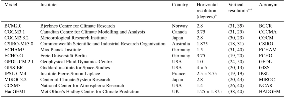
The Program for Climate Model Diagnosis and Inter-comparison (PCMDI) collected model results from GCM runs based on the IPCC SRES scenarios and made the re-sults available through the PCMDI data portal (https://esg. llnl.gov:8443/index.jsp). We selected the emission scenario A1B, which is positioned at the upper range of possible CO2 emissions. This rather extreme scenario was selected since for the period 2000 to 2006 observed CO2 emissions have been larger than estimated by models (Canadell et al., 2007; Global Carbon project, 2008). In addition the signal to noise ratio is relatively clear for an extreme scenario, especially for a time horizon of 2100. Complete datasets, with the required variables available on a daily time-step for both the 20C3M control experiment (1971–1990) and the A1B emission sce-nario (2081–2100), could be retrieved for twelve GCMs (see Table 1). Unfortunately the data availability restricted this analysis to these twelve GCMs, although a larger GCM en-semble would provide more information on uncertainty. Fur-thermore a longer period would have been better for aver-aging out inter-decadal variability. However, for the future experiments data were only available for a 30 yr period for some of the GCMs. Although the data portal does not pro-vide all required variables for the Hadley centre climate mod-els, HadGEM1 has been included for it is frequently used in climate change studies. HadGEM1 data has been retrieved from the CERA-gateway (http://cera-www.dkrz.de).
Table 1. Overview of selected GCMs.
Model Institute Country Horizontal Vertical Acronym
resolution resolution∗∗ (degrees)∗
BCM2.0 Bjerknes Centre for Climate Research Norway 2.8 (31, 35) BCCR
CGCM3.1 Canadian Centre for Climate Modelling and Analysis Canada 3.75 (31, 29) CCCMA
CGCM2.3.2 Meteorological Research Institute Japan 2.8 (30, 23) CGCM
CSIRO-Mk3.0 Commonwealth Scientific and Industrial Research Organization Australia 1.875 (18, 31) CSIRO
ECHAM5 Max Planck Institute Germany 1.5 (31, 40) ECHAM
ECHO-G Freie Universit¨at Berlin Germany 3.75 (19, 20) ECHO
GFDL-CM 2.1 Geophysical Fluid Dynamics Centre USA 1.0 (24, 50) GFDL
GISS-ER Goddard institute for Space Studies USA 4×5 (20, 13) GISS
IPSL-CM4 Institute Pierre Simon Laplace France 2.5×3.75 (19, 19) IPSL
MIROC3.2 Center of Climate System Research Japan 2.8 (20, 43) MIROC
CCSM3 National Center for Atmospheric Research USA 1.4 (26, 40) NCAR
HadGEM1 Met Office’s Hadley Centre for Climate Prediction UK 1.25×1.875 (38, 40) HADGEM
∗Parkinson et al. (2006);∗∗nr atmospheric layers, nr ocean layers
2.3 Statistical analysis 2.3.1 Statistics
To quantify the projected hydrological changes between the future and control experiments and the consistency of these changes, consistency maps were derived. In the following sections we describe how changes in these statistical quanti-ties are obtained from the multi-model ensemble and how the likelihood and consistency of the changes have been quantified.
2.3.2 Relative change
Discharge changes have been calculated relative to the base-line multi-model simulations. We did not look at absolute values, because the GCM precipitation and consequently the derived discharges deviate from observed quantities for some of the catchments (Van Beek et al., 2011). The relative changes for the two scenarios have been calculated for each model individually, according to the following equation:
1Qfuture = Qfuture −Qpast Qpast (1)
whereQcan be one of the statistics in Table 2, “past” refers to the 20C3M experiment and “future” refers to the A1B sce-nario. For the timing of peak discharges absolute changes were calculated. From the relative change fields per model (1Qi) we calculated maps with the ensemble mean change
(1Q) for the different statistics:
1Q = 1
12 12
X
i=i
1Qi. (2)
We prefer to work with a non weighted multi-model mean, since weights have to be derived from past performance and
may not hold for future periods because of apparent small persistence in relative model skill (Reifen and Toumi, 2009). The multi model ensemble, with equal weights assigned to each member, is likely to give good results and contains all the uncertainty information available. Furthermore, weight-ing on a limited number of indices of GCM performance may result in a misleading estimate of change, because the more complex picture of the relative merits of the individual GCMs is hidden (Gosling et al., 2011).
2.3.3 Likelihood and consistency
Notable discharge changes, between the 20th century climate control experiment and the A1B scenario for 2100, were de-rived for each GCM individually relative to its inter-annual variability. This was done by applying the independent sam-ples t-test. However, an inter-annual autocorrelation is ex-pected to exist in the yearly runoff time series, resulting in an effective decrease of the number of independent observa-tions. This dependency was accounted for by calculating the effective sample size from the lagged correlation coefficient, ρ, according to Matalas and Langbein (1962):
1 n∗b =
1 n +
2 n2
n−1
X
j=1
(n−j ) ρj 1t (3)
where1t is the observation interval (= 1 yr),n is the total number of observations andj 1t is the time lag for which the correlation coefficient is calculated. With this equation values ofn∗b (the effective sample size) were calculated for each model cell. Afterwards, independent two sample t-tests were conducted for each GCM individually using the effec-tive sample size.
t = Qfut −Qpast
Sfut past
q 1
n∗ fut
+ 1
n∗ past
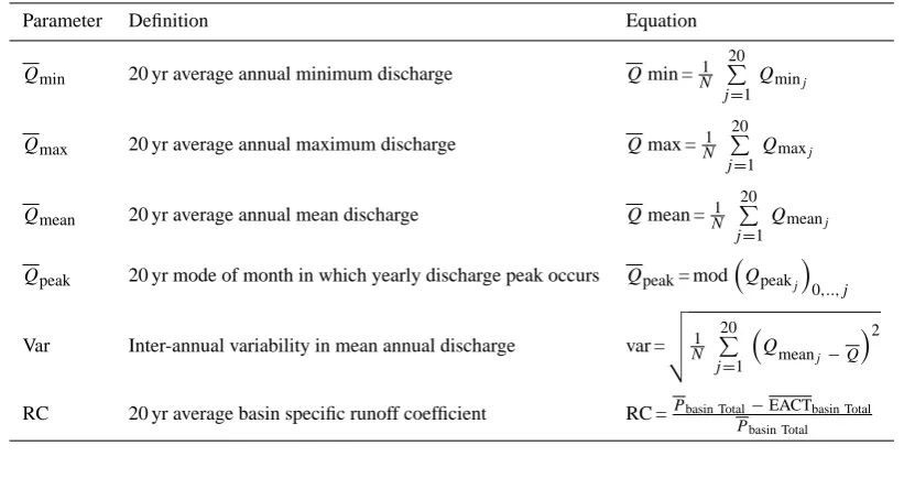
Table 2. Parameters included in analysis.Qmeanj,Qminj andQmaxj are respectively the mean, minimum and maximum daily discharge
of yearj. jis the year number and ranges from 1 to 20. N= 20, the total number of years. Qpeakj is the number of the month in which discharge peak occurred in yearj. Qis the twenty year mean discharge. Psumis the twenty year average annual basin total precipitation sum and EACTsumis the twenty year average annual basin total modeled actual evaporation sum.
Parameter Definition Equation
Qmin 20 yr average annual minimum discharge Qmin =N1
20 P
j=1
Qminj
Qmax 20 yr average annual maximum discharge Qmax =N1
20 P
j=1
Qmaxj
Qmean 20 yr average annual mean discharge Qmean =N1
20 P
j=1
Qmeanj
Qpeak 20 yr mode of month in which yearly discharge peak occurs Qpeak= mod
Qpeakj
0,..,j
Var Inter-annual variability in mean annual discharge var = v u u t1
N
20 P
j=1
Qmean
j−Q
2
RC 20 yr average basin specific runoff coefficient RC =Pbasin Total−EACTbasin Total Pbasin Total
Sfut past =
v u u u t
n∗fut−1S2fut+ n∗past −1Spast2
n∗fut +n∗past −2
(5)
whereSfut andSpast are respectively the standard deviation of yearly average minimum, maximum or mean discharge for the A1B scenario and the 20C3M experiment.QfutandQpast are the 20 yr average discharge statistics for the A1B scenario and control experiment and n∗fut andn∗past are the effective degrees of freedom as calculated with Eq. (6).
We assume the distribution of mean, maximum and min-imum discharge to be approximately Gaussian, a criterium that needs to be met for applying the above t-statistics. This criterium can not be met for the timing of peak discharge and inter-annual variability, therefore t-statistics are not cal-culated for these variables. In addition, discharges calcu-lated from data of a single GCM for the different time-slices can not be assumed to be completely random samples as the meteorological data are generated with the same GCM (von Storch, 1995). Still we apply the above t-statistics, although only to distinguish notable changes from noise.
To quantify the consistency in projected change between the twelve models, the number of models projecting notable change in the dominant direction (i.e. the direction of the mean of the multi-model ensemble) was calculated for each individual model cell. The resulting consistency maps indi-cate for which regions of the world the models project consis-tent changes in discharge and where consequently likelihood of discharge changes is higher than in other regions.
2.3.4 Annual cycle
To illustrate the changes in monthly flows and possible sea-sonal shifts, mean annual cycles have been derived for each catchment. In the first step, mean annual cycles were derived over the twenty year model run period for each model indi-vidually for both the 20C3M experiment and the A1B sce-nario. The two resulting sets of twelve GCM derived annual cycles gave for each month long-term average distributions of GCM derived discharge from which for the 20C3M ex-periment and A1B scenario individually the mean, 10th- and 90th-percentile discharges per month were calculated. By doing so the plots of the resulting annual regimes do not only give information on the changes in mean annual cycle, but also on the spread in the annual cycles obtained from the en-semble of models.
3 Results
Global maps with monthly mean discharge and actual and potential evaporation derived from the daily results of the GCM based hydrological model runs (e.g. hydrological sce-nario data) can be downloaded from: http://opendap.deltares. nl/thredds/dodsC/opendap/deltares/FEWS-IPCC.
3.1 Global patterns of change
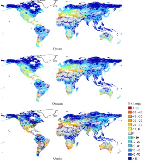
Qmax
Qmean
Qmin
[image:7.595.308.547.64.420.2]% change
Fig. 3. Maps showing the multi-model ensemble average
percent-age change (%) in the hydrological parameters annual maximum, minimum and mean discharge for the emission scenario A1B rela-tive to the 20C3M control experiment.
average annual mean daily discharge, minimum discharge is the average of the minimum daily discharge calculated for the twenty individual years and maximum is the average of the maximum daily discharge calculated for the twenty in-dividual years. The regions where minimum, maximum and mean discharge increase and decrease are the same, although regions with decreases are more extended for minimum dis-charge in the US and Eastern Europe and increases in max-imum discharge are larger in Arctic and Sub-Arctic regions. Similar global patterns of change can be found in literature (Alcamo et al., 2007; Milly et al., 2005; Nohara et al., 2006). Several studies (Alcamo and Henrichs, 2002; Arnell, 1999; V¨or¨osmarty et al., 2000) indicated large parts of the regions, for which we calculated discharge decreases, as areas cur-rently experiencing water stress. According to these studies, water stress will increase for most of these areas, depending on the definition of the water use scenario.
Figure 4 shows ensemble average seasonal discharge changes. Seasonal changes in precipitation, temperature and actual evaporation were derived as well to explain discharge changes. However, for briefness, maps resulting from these calculations have not been included. Maximum discharge increases are projected for the Arctic and sub-Artic regions and for south-east Asia. These increases are related to an increase of precipitation in the JJA and SON seasons. Fig-ure 4 shows that in North-Western Europe and the Eastern
DJF
MAM
JJA
SON
% change
Fig. 4. Multi-model ensemble average seasonal discharge changes
(%) for the scenario A1B as a percentage of the discharges cal-culated for the 20C3M control experiment. From top to bottom the seasons: December-January-February, March-April-May, June-July-August and September-October-November.
US winter runoff increases while summer runoff will de-crease. This mirrors changes in precipitation distribution over the year, with wetter boreal winters and drier boreal summers. Areas around the Mediterranean Sea, the south-west of South-America, parts of south and north Africa and the south of Australia experience discharge decreases caused by large precipitation decreases. In South Africa this precip-itation decrease is accompanied by an evaporation increase for the DJF and MAM season. The seasonal patterns of pre-cipitation and evaporation of the multi model mean show that during the summer (JJA) the African monsoon reaches fur-ther north which results in rainfall and discharge increases in the Northern Sahel.
[image:7.595.48.287.65.331.2]humid wetter
humid drier
arid wetter
[image:8.595.49.283.65.143.2]arid drier
Fig. 5. Change in aridity. The division in humid and arid regions is
obtained from the WWRDII climate moisture indices (UN, 2006). The globe is divided in humid regions becoming wetter (dark blue), humid regions becoming drier (light blue), arid regions becoming wetter (green) and arid regions becoming drier (yellow) based on the ensemble average change calculated for the A1B scenario.
ensemble mean projected changes (Fig. 3). For the arid re-gions; Southern Africa, the northern African coast, southern Australia, the southern US and Spain discharge decreases are projected. The more humid part of southern Europe will ex-perience discharge decreases, for most other humid world regions (e.g. southeast Asia, Arctic and sub-Arctic regions, eastern US, the Amazon) discharge increases are projected. Current dry regions for which discharge increases are pro-jected are northern Australia, parts of Asia, Russia and the centre of the US. For northern Africa discharge increases are projected as well, however in absolute values these increases are negligible.
Besides change in runoff quantities, maps with shift in timing of peak discharge were calculated by taking the dif-ference between the ensemble mode of the month of peak occurrence for the A1B scenario and the 20C3M experiment (Fig. 6). For large parts of the world, shifts are less than a month. There is a shift backward in time for most of the sub-Arctic regions. This shift is caused by increased temper-atures for the spring and summer season resulting in earlier snowmelt and more precipitation falling as rain. For parts of South-Asia a shift forward in peak timing of a half up to one month is calculated. This may result from a delay in the Monsoon rainfall that shifts from the JJA to the SON season, caused by a later reversal of the meridional tropospheric tem-perature gradient (Ashfaq et al., 2009). However the plots of the annual cycles of other Monsoon influenced rivers do not show this shift. For most southern parts of the world changes are mixed. And, although shifts in timing are also displayed for deserts and tropic regions, they contain limited informa-tion since precipitainforma-tion is relatively constant throughout the year in these regions and consequently the annual cycle has only a small amplitude.
3.2 Consistency on global patterns of change
[image:8.595.308.547.65.148.2]GCM consistency maps for change in the different hydrolog-ical variables are given in Figs. 7 and 8. In these figures, likelihood of change is quantified for the individual GCMs relative to the GCM specific 20 yr inter-annual variability.
Fig. 6. Map showing the number of months change in the timing
of peak discharge occurrence calculated by taking the mode of the ensemble of timings calculated for the twelve individual GCMs for the scenario A1B relative to to 20C3M control experiment.
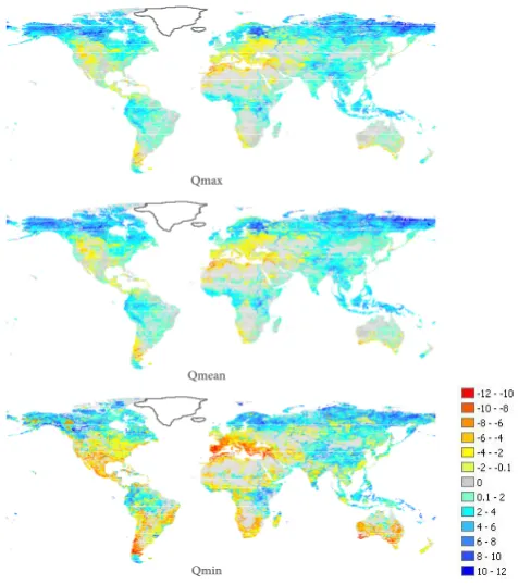
Qmax
Qmean
Qmin
Fig. 7. Maps showing the number of models projecting significant
change (for a significance level of 5 %) in the same direction as the ensemble mean direction of change (see Sect. 2.4 for more in-formation). From top to bottom the figure shows GCM consisten-cies for maximum, mean and minimum discharge. Negative values correspond to the number of models projecting discharge decrease, positive values correspond to the number of models projecting dis-charge increases, grey areas correspond to areas with no significant change.
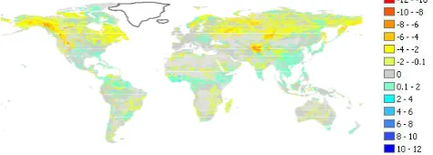
[image:8.595.308.547.221.490.2]Fig. 8. Maps showing the number of models projecting change in
timing of the annual cycle consistent with the ensemble mean di-rection of change of timing. The negative numbers correspond to the number of models projecting advances in the annual cycle con-sistent with the ensemble mean advances, positive numbers corre-spond to consistent projected delays in the timing of regime, grey areas correspond to regions with zero change.
minimum and especially maximum discharge than on change in mean discharge. Consensus on seasonal shift of peak dis-charge (Fig. 8) is large for sub-Arctic regions where temper-ature rise causes an earlier snow melt driven discharge peak. For dry areas the timing of peak is difficult to assess due to low discharge values and small amplitudes, therefore mod-els show little consensus on the direction of change in these regions.
3.3 Continental discharge changes
For each continent and each ocean the change in freshwater flowing into the oceans was calculated by summing the 20 yr average mean accumulated runoff of rivers discharging into the oceans (Fig. 9). For all continents discharge to oceans increases according to the ensemble mean change. This con-firms that there will be an intensification of the hydrological cycle (Huntington, 2006).
Discharge increases are smallest for Africa, Europe and South-America, as multiple GCMs also project discharge de-creases for large parts of these continents. In Australia and Africa, despite the continental discharge increases, the ef-fects of discharge decreases are large since they mainly oc-cur in regions that are already arid at this stage (see in Fig. 5 the projected decreases in the arid regions of southern Africa and southern Australia including the Murray basin). Inflow to the oceans will increase for all oceans except the Mediter-ranean Sea. Inflow to the MediterMediter-ranean Sea originates from Southern Europe and Northern Africa, both regions with pro-jected discharge decreases. Large discharge decreases for the Mediterranean region, up to 40 %, have also been found by Sanchez-Gomez et al. (2009).
The spread in projected changes is smallest for Europe and South-America. Here discharge increases and decreases pro-jected by the individual GCMs are small and the resulting ensemble mean projected change is close to zero. For the other continents ensemble mean change as well as the ensem-ble uncertainty is larger. For Australia and Asia a consistent
discharge increase is projected and, although for Africa and North-America increases are projected as well, the ensem-ble mean change is smaller as some GCMs project discharge decreases.
Globally we find an ensemble mean discharge increase of 11.0 % by 2100. In contrast, Arnell (1999) found a slight decrease for the HadCM2 ensemble; by 2080 an ensemble mean decrease of mean discharge from−0.4 %. Although three of the four individual ensemble members of his en-semble gave a discharge increase ranging between 0.6 and 1.0 %. For the HadCM3 model he found a decrease of
−14.7 %. This illustrates the large differences amongst mod-els. V¨or¨osmarty et al. (2000) found a global discharge de-crease of−5.6 % for their time horizon of 2025 and Arora and Boer (2001) found a larger decrease of−14 % by the end of the 21st century. These differences might be a re-sult of the use of the previous version of IPCC scenarios. However, more likely they are a result of the uncertainty be-tween GCMs. Even for global average changes in tempera-ture there is less variance amongst selected emission scenar-ios than amongst projections obtained from different GCMs. Depending on the selected scenario, the ensemble range of projected temperature ranges from 1.5 to 3◦K (Kelvin) or 2 to 4.5◦K. While the absolute projected global tempera-ture changes is on average 2◦K temperature increase for the 1 % CO2increase scenario Arnell (1999) used, 3 K increase for the IS92a scenario Arora and Boer (2001) followed and 3 K increase for the A1B scenario used in this study (IPCC, 2007). GCM ensemble uncertainty ranges for projected pre-cipitation ranges are even larger (see Table 3).
3.4 Catchment results
Mean annual discharge cycles of the selected river basins are shown in Fig. 10 for the control experiment 20C3M, the A1B scenario and for discharge observations. Furthermore per-centage changes in 20 yr average minimum, maximum, mean discharge and runoff coefficient, absolute changes in timing of peak discharge, and changes in variability are shown in Table 4. Variations between the individual GCMs are large and changes in discharge projected by individual GCMs are even contradictory for certain catchments.
(a) (b)
Fig. 9. (a) Continental discharge changes (%), (b) change in freshwater inflow to oceans (%). Vertical bars represent range of changes
[image:10.595.52.546.61.207.2]covered by the entire ensembles of GCMs, large horizontal dashes represent ensemble mean change, small horizontal dashes represent minimum and maximum projected changes.
Table 3. Change in global temperature (K), precipitation (%) and discharge (%) for different emissions scenarios.
Temperature Ensemble Ensemble Ensemble Horizon Source min mean max
1 % CO2 1.5 2 3 2100 Andrews and Forster (2010) IS92a 2 3 4.5 2100 IPCC (2007)
A1B 2 3 4.5 2100 IPCC (2007)
Precipitation
1 % CO2 2 4 6 2100 Andrews and Forster (2010) IS92a 1.5 4 6 2100 IPCC (2007)
A1B 1.5 4.5 7 2100 IPCC (2007)
Discharge
1 % CO2 −14.7 −0.4 1 2080 Arnell (1999) IS92a −14 2100 Arora and Boer (2001)
A1B −7 11 28 2100 This study
of Nijssen et al. (2001) for the Yellow river. This is a result of difference in GCMs used and differences in selected emis-sion scenarios, which is probably of minor relevance given the large uncertainty between GCMs.
A decrease in mean discharge is projected for the African rivers; Zambezi, Orange and Niger. Furthermore the Zam-bezi shows a decrease of the 10-percentile of ensemble discharge towards no flow. Especially for the south of Africa, estimated precipitation decreases are large. The dis-charge decreases are in agreement with results of Arora and Boer (2001) who calculated a decrease of mean annual dis-charge for the warmer world and Nohara et al. (2006), who found decreases for the African rivers. For the Orange river the large decrease in discharge results in a related ensemble mean decrease of inter-annual discharge variability.
For the Lena and Mackenzie a large discharge increase was estimated, which is related to earlier snowmelt due to higher temperatures and a calculated increase in precipita-tion for the SON season that is stored during winter as snow.
Nijssen et al. (2001) and Nohara et al. (2006) calculated an advance in peak for Arctic rivers, which can also be seen form our annual cycle plots. Arora and Boer (2001) also found an advance in phase for the high-latitude rivers and an increase in amplitude.
[image:10.595.118.475.275.456.2]Fig. 10. Modeled annual hydrological cycles for the 19 selected catchments, showing for each experiment the monthly 20-yr average
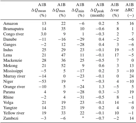
Table 4. Percentage change for the hydrological parameters of
in-terest (see Table 3). Calculated for the A1B experiment, relative to the 20C3M experiment.
A1B A1B A1B A1B A1B A1B
1Qmean 1Qmax 1Qmin 1Qpeak 1var 1RC
(%) (%) (%) (month) (%) (−)
Amazon 13 22 −6 0.2 5 16
Bramaputra 14 35 10 −0.6 8 1
Congo river 3.0 9 1 −0.3 2 7
Danube −11 −16 −29 0.4 −2 −6
Ganges −2 12 −28 0.4 3 −6
Indus 25 29 23 −0.1 19 −5
Lena 21 47 11 −0.1 17 −5
Mackenzie 28 36 25 −0.5 7 0
Mekong 21 52 9 0.6 3 13
Mississippi −5 5 −17 0.2 3 −10
Murray river −14 0 −23 −0.1 0 24
Niger −53 19 ∗ −0.3 4 −10
Orange river −10 5 −24 1.3 −5 5
Parana 4 9 −28 0.3 −3 19
Rhine −2 4 −31 −0.5 8 −1
Volga 21 19 23 −0.1 14 −4
Yangtze 14 23 19 0.2 4 0
Yellow river 19 33 22 −0.1 10 −1
Zambezi −3 −6 ∗ −0.7 −2 14
∗The minimum flow in the Zambezi and Niger becomes zero for several GCMs for the
future climate therefore % changes are omitted here.
Large discharge decreases are likely for the Danube. Pre-cipitation decreases are large in both the Danube and the Rhine basin in particular for the summer period. Discharge of the Rhine overall decreases but there is an increase in max-imum discharge. This is related to the calculated tempera-ture increases, leading to earlier snowmelt and an increased amount of spring precipitation falling as rain instead of snow which enters the river earlier in the year. The study of No-hara et al. (2006) showed a decrease in discharge for the river Danube and Rhine as well. However, again there is a dif-ference with Aerts et al. (2006) who found little change in Danube discharge.
3.5 Change in catchment specific runoff coefficients To quantify the relative change in water balance partition-ing due to climate change, the change in runoff coefficients (RC; for the definition see Table 2) has been calculated for all individual catchments for the selected measurement stations (see percentage changes in the last column Table 4). For the calculations, twenty year average year sums of accumulated upstream precipitation and actual evaporation have been used to avoid the influence of storage changes in glaciers and soil water. Basins with an increase of RC of more than 10 % are the Amazon, Parana, Murray, Zambezi, Mississippi and Mekong. For the Mekong this increase is caused by an crease in precipitation. The Parana also experiences an in-crease in precipitation together with a dein-crease of actual evaporation. For the Murray and Zambezi the decrease in
actual evaporation is larger than the decrease in precipita-tion, also resulting in increasing RC. Except for the Niger, the African rivers all have an increasing runoff coefficient, indicating that the part of precipitation that evaporates de-creases. The Niger is the only basin with a decrease in RC of more than 10 %. This decrease is caused by small changes in precipitation and large evaporation increases. The runoff coefficient decreases for the Danube and Rhine (slight de-crease), due to a decreasing amount of precipitation and be-cause a larger part of the precipitation will evaporate due to temperature increases.
4 Discussion
In an attempt to make an as complete as possible assessment of the global hydrological effects of climate change we pro-vided and overview of previous hydrological studies and pre-sented our results in the context of the previous results. We used a, for global scale hydrological studies, relatively large ensemble of GCMs existing of all the GCMs for which the PCMDI data portal provided the required daily time-series of meteorological variables which were needed as input to the hydrological model. We estimated changes in spatial and temporal discharge variability and calculated the ensemble consistency of the projected changes. In addition to previ-ous studies we quantified likelihood of change relative to the individual GCM inter-annual variability. By using this alter-native analyses of calculating likelihood of change relative to the GCMs inter-annual variability, it is possible to denote regions with notable change, despite the uncertainty between models.
Although using an ensemble of GCMs for the estima-tion of future change is often recommended (Boorman and Sefton, 1997; Murphy et al., 2004) previous studies also crit-icized the use of the ensemble mean change (Materia et al., 2010). By averaging the results of multiple GCMs extremes are reduced, discharge cycles are smoothened and changes become less pronounced. Still, by using multiple models, all available information is considered in the analysis, the influence of discrepancies in single models is reduced and model uncertainties can be analyzed. In addition, by inves-tigating the ensemble consistency, regions with large uncer-tainties and discrepancies between models are identified.
best available means for assessing future changes (Pielke et al., 2009; Beven, 2011).
From an evaluation of the 12 GCMs on the reproduction of the annual discharge cycles and hydrological extremes for the catchments included in this analysis, we concluded that for each basin other GCMs perform best and a sub-set which outperforms the other GCMs for all basins and hydrological variables included in this analysis does not exist. Therefore the full ensemble was used.
Furthermore, it should be noted that the hydrological model introduces uncertainties as well, amongst others due to structural simplifications and parameter uncertainties and the absence of anthropogenic influences as for example wa-ter use and river regulation in the routing scheme (Sperna Weiland et al., 2010; Van Beek et al., 2011; Vrugt et al., 2003). For a full uncertainty assessment, multiple hydrolog-ical models should be employed here. Unfortunately, such a study quickly becomes unfeasible. Here, we restricted our-selves to a multiple GCM analysis as Gosling et al. (2011) already stated in their multi- hydrological and climate model comparison for multiple basins around the world, that the range in projections from different hydrological models is smaller than the range of projections from different GCMs.
This study is restricted to hydrological changes due to cli-mate change, for a full assessment of future water availability the impact of climate change on hydrological change should be placed in light of other factors as for example population growth, land use change and water management. The im-pact of these factors may be comparable or larger than the impact of climate change (Beven, 2011; Pielke et al., 2009; V¨or¨osmarty et al., 2000; Alcamo et al., 2007; Arnell, 2004). The result of this study show that river discharge will in-crease for the Yangtze, Yellow river, Mekong, Ganges, In-dus and Brahmaputra due to an increase in monsoon rainfall. As a result of earlier snowmelt and an increase of precipi-tation the Lena and MacKenzie show an increase in spring discharge and a small shift in timing of peak. A decrease in both mean and extreme discharge is projected for the Orange, Niger, Murray and Danube. Comparable results have been found in previous studies especially when looking at global patterns of change, but differences exist both on catchment and continental scale.
Changes in the downstream part of the river basins and especially in the main river courses are often more likeliy than the changes for grid cells located upstream in the catch-ment. This may be because variations in climate patterns are accumulated downstream. It confirms the importance of dis-charge accumulation and the use of a routing scheme that, although biases are present for several catchments, allows for temporal storages in lakes and reservoirs and introduces realistic travel times which are especially relevant in larger catchments like the Amazon (Sperna Weiland et al., 2011).
The climate models do not always project consistent changes, especially for areas with temperate climate. In ad-dition to the information on the discharge change maps, the
consistency maps (Fig. 7) indicate the agreement amongst models on the direction of significant change in relation to inter-annual variability and thereby give an indication of re-gions where discharge is likely to be affected by climate change. Such an analysis partly accounts for the influence of GCM model errors and may be the preferred change de-tection method for grid-based global assessment of discharge change.
According to the ensemble mean calculations, continental outflow to oceans will increase for all oceans except for the Mediterranean Sea. The GCMs project a consistent decrease in runoff for southern Europe, South Australia, South Africa, parts of north Africa and the southwestern coast of South-America. There is also large consensus on discharge increase for the Arctic regions and the Northern Sahel. Besides these results, the following three findings are useful to hydrolog-ical climate effect studies in general. First, we found that the projected changes in our study show the largest differ-ences with studies based on a small number of climate mod-els. When using only small ensembles the response may be biased through the influence of only one or two GCMs that deviate from the other models, while in larger ensemble these deviating GCMs will have less influence due to the averaging of multiple change projections. This underscores the value of using large ensembles. Second, from the differences with the study of Aerts et al. (2006) it can be concluded that choice of the reference period influences the change signal. Aerts et al. (2006) used data for the period 1750 to 2000 as a reference for the change projections and to investigate the influence of interdecadal variability. When using a reference period of this length the influence of inter-annual variability is mini-mized, whereas in our twenty year period it is more likely that the average discharge is disturbed by effects like El Nino. Furthermore, in this study change is calculated between 2100 and the time-slice 1961–1990, which is likely to represent current climate conditions. Whereas Aerts et al. (2006) cal-culated change relative to the period 1750–2000 and changes will therefore either be relatively large or less extreme due to long-term variations in the climate that resemble future cli-mate changes. Third and finally, our results are comparable to studies using the change factor method which, for compu-tational reasons, might therefore be the preferable method to use.
5 Conclusions
projected for sub-Arctic and Arctic regions and an advance in phase in the annual cycle is projected for the sub-Arctic regions. Overall, discharge of Monsoon influenced rivers slightly increases.
The results of this study are generally comparable to pre-vious studies. Although, results of studies using only a small number of GCMs show relatively large differences from our study and the use of a multi-model ensemble is therefore preferable. We illustrated that by considering the consistency of change amongst models (i.e. in light of the likelhood of projected change relative to natural variability) regions with high likelihood of changes in the annual cycle can clearly be revealed.
Supplementary material related to this article is available online at:
http://www.hydrol-earth-syst-sci.net/16/1047/2012/ hess-16-1047-2012-supplement.pdf.
Acknowledgements. We acknowledge the GCM modeling groups, the Program for Climate Model Diagnosis and Intercomparison (PCMDI) and the WCRP’s Working Group on Coupled Modelling (WGCM) for their roles in making available the WCRP CMIP3 multi-model dataset. Support of this dataset is provided by the Office of Science, US Department of Energy. We would like to thank the reviewers, R. T. Clarke, B. Fekete, S. Materia and G. A. Corzo, for their extensive review comments which greatly helped us to improve the quality of this manuscript.
Edited by: J. Liu
References
Aerts, J., Renssen, H., Ward, P. J., de Moel, H., Odada, E., Bouwer, L. M., and Goosse, H.: Sensitivity of global river discharges un-der Holocene and future climate conditions, Geophys. Res. Lett., 33, L19401, doi:10.1029/2006GL027493, 2006.
Alcamo, J. and Henrichs, T.: Critical regions: A model-based es-timation of world water resources sensitive to global changes, Aquat. Sci., 64, 1–11, 2002.
Alcamo, J., Fl¨orke, M., and M¨arker, M.: Future long-term changes in global water resources driven by socio-economic and climatic changes, Hydrolog. Sci. J., 52, 247–275, 2007.
Allen, R. G., Pereira, L. S., Raes, D., and Smith, M.: Crop evapo-transpiration: FAO Irrigation and drainage paper 56, FAO, Rome, Italy, 1998.
Andrews, T. and Forster, P. M.: The transient response of global-mean precipitation to increasing carbon dioxide levels, Environ. Res. Lett., 5, 025212, doi:10.1088/1748-9326/5/2/025212, 2010. Arnell, N. W.: Climate change and global water resources, Global
Environ. Change, 9, 831–849, 1999.
Arnell, N. W.: Effects of IPCC SRES* emissions scenarios on river runoff: a global perspective, Hydrol. Earth Syst. Sci., 7, 619– 641, doi:10.5194/hess-7-619-2003, 2003.
Arnell, N. W.: Climate change and global water resources: SRES emissions and socio-economic scenarios, Global Environ. Change, 14, 31–52, doi:10.1016/j.gloenvcha.2003.10.006, 2004.
Arora, V. K. and Boer, G. J.: Effects of simulated climate change on the hydrology of major river basins, J. Geophys. Res., 106, 3335–3348, 2001.
Ashfaq, M., Shi, Y., Tung, W., Trapp, R. J., Gao, X., Pal, J. S., and Diffenbaugh, N. S.: Suppression of south Asian summer mon-soon precipitation in the 21st century, Geophys. Res. Lett., 36, L01704, doi:10.1029/2008GL036500, 2009.
Beven, K.: I believe in climate change cut how precautionary do we need to be in planning for the future, Hydrol. Process., 25, 1517–1520, doi:10.1002/hyp.7939, 2011.
Bierkens, M. F. P. and Van Beek, L. P. H.: Seasonal predictability of european discharge: NAO and hydrological response time, J. Hydrometeorol., 10, 953–968, 10.1175/2009JHM1034.1, 2009. Boorman, D. B. and Sefton, C. E. M.: Recognizing the uncertainty
in the quantification of the effects of climate change on hydro-logical response, Climatic Change, 35, 415–434, 1997. Brouwer, C. and Heibloem, M.: Irrigation water management:
Irri-gation water needs, FAO, Rome, Italy, 1986.
Canadell, J. G., Le Qu´er´e, C., Raupach, M. R., Field, C. B., Buite-huis, E. T., Ciais, P., Conway, T. J., Houghton, R. A., and Mar-land, G.: Contributions to accelerating atmospheric CO2growth from economic activity, carbon intensity, and efficiency of natu-ral sinks, P. Natl. Acad. Sci., 104, 18866–18870, 2007.
Covey, C., AchutaRao, K. M., Cubasch, U., Jones, P., Lam-bert, S. J., Mann, M. E., Phillips, T. J., and Taylor, K. E.: An overview of results from the coupled model in-tercomparison project, Global Planet. Change, 37, 103–133, doi:10.1016/S0921-8181(02)00193-5, 2003.
D¨oll, P. and Lehner, B.: Validating of a new global 30-minute drainage direction map, J. Hydrol., 258, 214–231, 2002. Fowler, H. J., Blenkinsop, S., and Tebaldi, C.: Review: Linking
climate change modelling to impact studies: recent advances in downscaling techniques for hydrological modeling, Int. J. Clima-tol., 27, 1547–1578, doi:10.1002/joc.1556, 2007.
Giorgi, F. and Mearns, L. O.: Calculation of average, uncertainty range, and reliability of regional climate changes from AOGCM simulations via the “Reliability Ensemble Averageing” (REA) method, J. Climate, 15, 1141–1158, 2002.
Global Carbon Project Carbon budget and trends 2007: http://www. globalcarbonproject.org, last access: 26 September 2008. Gosling, S. N., Taylor, R. G., Arnell, N. W., and Todd, M. C.: A
comparative analysis of projected impacts of climate change on river runoff from global and catchment-scale hydrological mod-els, Hydrol. Earth Syst. Sci., 15, 279–294, doi:10.5194/hess-15-279-2011, 2011.
GRDC: Major River Basins of the World/Global Runoff Data Cen-tre, D – 56002, Federal Institute of Hydrology (BfG), Koblenz, Germany, 2007.
Huntington, T. G.: Evidence for intensification of the global water cycle: Review and synthesis, J. Hydrol., 319, 83–95, 2006. Immerzeel, W. W., Van Beek, L. P. H., and Bierkens, M. F. P.:
Cli-mate change will affect the Asian water towers, Science, 328, 1382–1385, doi:10.1126/science.1183188, 2010.
Kay, A. L. and Davies, V. A.: Calculating potential evaporation from climate model data: A source of uncertainty for hydrologi-cal climate change impacts, J. Hydrol., 358, 221–239, 2008. Kingston, D. G., Todd, M. C., Taylor, R. G., and Thompson, J.
R.: Uncertainty in the estimation of potential evapotranspira-tion under climate change, Geophys. Res. Lett., 36, L20403, doi:10.1029/2009GL040267, 2009.
Lehner, B. and D¨oll, P.: Development and validation of a global dataset of lakes, reservoirs and wetlands, J. Hydrol., 296, 1–22, 2004.
Liu, J., Fritz, S., Van Wesenbeeck, C. F. A., Fuchs, M., You, L., Obersteiner, M., and Yang, H.: A spatially explicit assessment of current and future hotspots of hunger in Sub-Saharan Africa in the context of global change, Global Planet. Change, 64, 222– 235, 2008.
Liu, J., Zehnder, A. J. B., and Yang, H.: Global consump-tive water use for crop production: The importance of green water and virtual water, Water Resour. Res., 45, W05428, doi:10.1029/2007WR006051, 2009.
Matalas, N. C. and Langbein, W. B.: Information content of the mean, J. Geophys. Res., 67, 3441–3448, 1962.
Materia, S., Dirmeyer, P. A., Guo, Z., Alessandri, A., and Navarra, A.: The sensitivity of simulated river discharge to land surface representation and meteorological forcings, J. Hydrometeorol., 11, 334–351, 2010.
Meehl, G. A. and Arblaster, J. M.: Mechanisms for projected future changes in south Asian monsoon precipitation, Clim. Dynam., 21, 659–675, doi:10.1007/s00382-003-0343-3, 2003.
Meehl, G. A., Zwiers, F., Evans, J., Knutson, T., Mearns, L., and Whetton, P.: Trends in extreme weather and climate events: is-sues related to modelling extremes in projections of future cli-mate change, B. Am. Meteorol. Soc., 81, 427–436, 2000. Milly, P. C. D., Dunne, K. A., and Vecchia, A. V.: Global pattern of
trends in streamflow and water availability in a changing climate, Nature, 438, 347–350, doi:10.1038/nature04312, 2005. Monteith, J. L.: Evaporation and environment, Symp. Soc. Exp.
Biol., 19, 205–234, 1965.
Murphy, J. M., Sexton, D. M. H., Barnett, D. N., Jones, G. S., Webb, M. J., Collins, M., and Stainforth, D. A.: Quantification of mod-elling uncertainties in a large ensemble of climate change simu-lations, Nature, 430, 768–772, 2004.
New, M., Hulme, M., and Jones, P.: Representing Twentieth-Century space-time climate variability, Part 1: Development of a 1961–90 mean monthly terrestrial climatology, J. Climate, 12, 829–856, 2000.
Nijssen, B., O’Donnel, G. M., Hamlet, A. F., and Lettenmaier, D. P.: Hydrologic sensitivity of global rivers to climate change, Cli-matic Change, 50, 143–175, 2001.
Nohara, D., Kitoh, A., Hosaka, M., and Oki, T.: Impact of climate change on river discharge projected by multimodel ensemble, J. Hydrometeorol., 7, 1076–1089, 2006.
Oki, T. and Kanae, S.: Global hydrological cycles and world water resources, Science, 313, 1068–1072, 2006.
Oudin, L., Hervieu, F., Michel, C., Perrin, C., Andr´eassian, V., An-ctil, F., and Loumagne, C.: Which potential evapotranspiration input for a lumped rainfall-runoff model? Part 2 – Towards a sim-ple and efficient potential evapotranspiration model for rainfall-runoff modeling, J. Hydrol., 303, 290–306, 2005.
Parkinson, C. L., Vinnikov, K. Y., and Cavalieri, D. J.: Evaluation of the simulation of the annual cycle of Arctic and Antarctic sea ice coverages by 11 major global climate models, Geophys. Res. Lett., 111, C07012, doi:10.1029/2005JC003408, 2006.
Pielke, R., Beven, K. J., Brasseur, G., Calvert, J., Chahine, M., Dickerson, R., Entekhabi, D., Foufoula-Georgiou, E., Gupta, H., Gupta, V., Krajewski, W., Krider, E. P., Lau, W. K. M., McDon-nell, J. J., Rossow, W., Schaake, J., Smith, J., Soroosh, S., and Wood, E. F.: Climate change: the need to consider human forc-ings other than greenhouse gases, EOS, Transactions-American Geophysical Union, 90, 413 pp., 2009.
Reifen, C. and Toumi, R.: Climate projections: past performance no guarantee of future skill, Geophys. Res. Lett., 36, L13704, doi:10.1029/2009GL038082, 2009.
Sanchez-Gomez, E., Somot, S., and Mariotti, A.: Future change in the Mediterranean water budget projected by an ensemble of regional climate models, Geophys. Res. Lett., 36, L21401, doi:0.1029/2009GL040120, 2009.
Sperna Weiland, F. C., van Beek, L. P. H., Kwadijk, J. C. J., and Bierkens, M. F. P.: The ability of a GCM-forced hydro-logical model to reproduce global discharge variability, Hy-drol. Earth Syst. Sci., 14, 1595–1621, doi:10.5194/hess-14-1595-2010, 2010.
Sperna Weiland, F. C., Van Beek, L. P. H., Kwadijk, J. C. J., and Bierkens, M. F. P.: On the suitability of GCM runoff fields for river discharge modeling; a case study using model output from HadGEM2 and ECHAM5, J. Hydrometeorol., 13, 140–154, doi:10.1175/JHM-D-10-05011.1, 2011.
UN: 2nd UN World Water Development Report: WWDRII data download page, http://wwdrii.sr.unh.edu/download.html (last ac-cess: November 201), 2006.
Uppala, S. M., K˚allberg, P. W., Simmons, A. J., Andrae, U., da Costa Bechtold, V., Fiorino, M., Gibson, J. K., Haseler, J., Her-nandez, A., Kelly, G. A., Li, X., Onogi, K., Saarinen, S., Sokka, N., Allan, R. P., Andersson, E., Arpe, K., Balmaseda, M. A., Beljaars, A. C. M., van de Berg, L., Bidlot, J., Bormann, N., Caires, S., Chevallier, F., Dethof, A., Dragosavac, M., Fisher, M., Fuentes, M., Hagemann, S., H´olm, E., Hoskins, B. J., Isak-sen, L., JansIsak-sen, P. A. E. M., Jenne, R. A., McNally, P., Mahfouf, J.-F., Morcrette, J.-J., Rayner, N. A. R., Saunders, W., Simon, P., Sterl, A., Trenberth, K. E., Untch, A., Vasiljevic, D., Viterbo, P., and Woollen, J.: The ERA-40 re-analysis, Q. J. Roy. Meteorol. Soc., 131, 2961–3012, 2005.
Van Beek, L. P. H.: Forcing PCR-GLOBWB with CRU mete-orological data, http://vanbeek.geo.uu.nl/suppinfo/vanbeek2008. pdf, last access: November 2011, Utrecht University, Utrecht, The Netherlands, 2008.
Van Beek, L. P. H. and Bierkens, M. F. P.: The Global Hy-drological Model PCR-GLOBWB: Conceptualization, Param-eterization and Verification, Report Department of Physical Geography: available at: http://vanbeek.geo.uu.nl/suppinfo/ vanbeekbierkens2009.pdf, last access: November 2011, Utrecht University, Utrecht, The Netherlands, 2009.
Viviroli, D., Archer, D. R., Buytaert, W., Fowler, H. J., Greenwood, G. B., Hamlet, A. F., Huang, Y., Koboltschnig, G., Litaor, M. I., L´opez-Moreno, J. I., Lorentz, S., Sch¨adler, B., Schreier, H., Schwaiger, K., Vuille, M., and Woods, R.: Climate change and mountain water resources: overview and recommendations for research, management and policy, Hydrol. Earth Syst. Sci., 15, 471–504, doi:10.5194/hess-15-471-2011, 2011.
V¨or¨osmarty, C. J., Green, P., Salisbury, J., and Lammers, R. B.: Global water resources: Vulnerability from climate change and population growth, Science, 289, 284–288, 2000.
Von Storch, H.: Misuses of statistical analysis in climate research, in: Analysis of Climate Variability: Applications of Statisti-cal Techniques, edited by: von Storch, H. And Navarra, A., Springer-Verlag, Berlin, 11–26, 1995.