https://doi.org/10.5194/hess-21-3071-2017 © Author(s) 2017. This work is distributed under the Creative Commons Attribution 3.0 License.
Rainfall and streamflow sensor network design: a review of
applications, classification, and a proposed framework
Juan C. Chacon-Hurtado1, Leonardo Alfonso1, and Dimitri P. Solomatine1,2
1Department of Integrated Water Systems and Governance, UNESCO-IHE, Institute for Water Education, Delft, the Netherlands
2Water Resources Section, Delft University of Technology, Delft, the Netherlands Correspondence to:Juan C. Chacon-Hurtado ([email protected]) Received: 20 July 2016 – Discussion started: 13 September 2016
Revised: 30 January 2017 – Accepted: 23 March 2017 – Published: 28 June 2017
Abstract. Sensors and sensor networks play an important role in decision-making related to water quality, operational streamflow forecasting, flood early warning systems, and other areas. In this paper we review a number of existing applications and analyse a variety of evaluation and design procedures for sensor networks with respect to various crite-ria. Most of the existing approaches focus on maximising the observability and information content of a variable of inter-est. From the context of hydrological modelling only a few studies use the performance of the hydrological simulation in terms of output discharge as a design criterion. In addi-tion to the review, we propose a framework for classifying the existing design methods, and a generalised procedure for an optimal network design in the context of rainfall–runoff hydrological modelling.
1 Introduction
Optimal design of sensor networks is a key procedure for im-proved water management as it provides information about the states of water systems. As the processes taking place in catchments are complex and the measurements are lim-ited, the design of sensor networks is (and has been) a rel-evant topic since the beginning of the International Hydro-logical Decade (1965–1974, TNO, 1986) until today (Pham and Tsai, 2016). During this period, the scientific commu-nity has not yet arrived at an agreement about a unified methodology for sensor network design due to the diver-sity of cases, criteria, assumptions, and limitations. This is evident from the range of existing reviews on hydrometric
network design, such as those presented by WMO (1972), TNO (1986), Nemec and Askew (1986), Knapp and Mar-cus (2003), Pryce (2004), NRC (2004), and Mishra and Coulibaly (2009).
The design of rainfall and streamflow sensor networks de-pends to a large extent on the scale of the processes to be monitored and the objectives to address (TNO, 1986; Loucks et al., 2005). Therefore, the temporal and spatial resolu-tion of measurements are driven by the measurement ob-jectives. For example, information for long-term planning does not require the same level of temporal resolution as for operational hydrology (WMO, 2009; Dent, 2012). On the global and country scale, sensor networks are commonly used for climate studies and trend detection (Cihlar et al., 2000; Grabs and Thomas, 2002; WMO, 2009; Environment Canada, 2010; Marsh, 2010; Whitfield et al., 2012), and are denoted as National Climate Reference Networks (WMO, 2009). On a regional or catchment scale, applications require careful selection of monitoring stations, since water resource planning and management decisions, such as operational hy-drology and water allocation, require high temporal and spa-tial resolution data (Dent, 2012).
project (www.wesenseit.eu), and the validation of the pro-posed methodology will be presented in subsequent publica-tions. This review does not consider in situ installation re-quirements or recommendations, so the reader is referred to WMO (2008a) for the relevant and widely accepted guide-lines, and to Dent (2012) for current issues in practice.
The structure of this paper is as follows: first, a classifi-cation of sensor network design approaches according to the explicit use of measurements and models is presented, in-cluding a review of existing studies. Next, a second way of classification is suggested, which is based on the classes of methods for sensor network analysis, including statistics, in-formation theory, case-specific recommendations, and oth-ers. Then, based on the reviewed literature, an aggregation of approaches and classes is presented, identifying potential op-portunities for improvement. Finally, a general procedure for the optimal design of sensor networks is proposed, followed by conclusions and recommendations.
1.1 Main principles of network design
The design of a sensor network uses the same concepts as experimental design (Kiefer and Wolfowitz, 1959; Fisher, 1974). The design should ensure that the data are sufficient and representative, and can be used to derive the conclusions required from the measurements (EPA, 2002), or to assess the water status of a river system (EC, 2000). In the context of rainfall–runoff hydrological modelling, provide the sufficient data for accurate simulation and forecasting of discharge and water levels, at stations of interest.
The objectives of the sensor network design have been cat-egorised into two groups, the optimality alphabet (Fedorov, 1972; Box, 1982; Fedorov and Hackl, 1997; Pukelsheim, 2006; Montgomery, 2012), which uses different letters to name different design criteria, and the Bayesian framework (Chaloner and Verdinelli, 1995; DasGupta, 1996). The alpha-betic design is based on the linearisation of models, optimis-ing particular criteria of the information matrix (Fedorov and Hackl, 1997). Bayesian methods are centred on principles of decision-making under uncertainty, in which it seeks to max-imise the gain in information (Shannon, 1948) between the prior and posterior distributions of parameters, inputs, or out-puts (Lindley, 1956; Chaloner and Verdinelli, 1995). Among the most used alphabetic objectives are the D-optimal, which minimises the area of the uncertainty ellipsoids around the model parameters, and G-optimal, which minimises the vari-ance of the predicted variable, which can also be used as ob-jective functions in the Bayesian design.
These general objectives are indirectly addressed in the literature of optimisation of hydrometric sensor networks, achieved by the use of several functional alternatives. These approaches do not consider block experimental design (Kirk, 2009), due to the incapacity to replicate initial conditions in a non-controlled environment, such as natural processes.
On the practical side, the design of a sensor network should start with the institutional set-up, purposes, objec-tives, and priorities of the network (Loucks et al., 2005; WMO, 2008b). From the technical point of view, an opti-mal measurement strategy requires the identification of the process, for which data are required (Casman et al., 1988; Dent, 2012). Considering that the information objectives are not unique and consistent or that the characterisation of the processes is not complete, the re-evaluation of the sensor net-work design should occur on a regular basis. Therefore, the sensor network should be re-evaluated when the studied pro-cess, information needs, information use, or modelling ob-jectives change. Consequently, regulations regarding moni-toring activities are often strict not in terms of station density, but in the suitability of data for providing information about the status of the water system (EC, 2000; EPA, 2002).
The design of meteorological and hydrometric sensor networks should consider at least three aspects. First, it should meet various objectives that are sometimes conflicting (Loucks et al., 2005; Kollat et al., 2011). Second, it should be robust in the event of failure of one or more measurement sta-tions (Kotecha et al., 2008). Third, it must take into account different purposes and users with different temporal and spa-tial scales (Singh et al., 1986). Therefore, the design of an op-timal sensor network is a multi-objective problem (Alfonso et al., 2010b).
The sensor network design can also be seen from an eco-nomic perspective (Loucks et al., 2005). In most cases, the main limitation in the deployment of sensor networks is re-lated to costs, being sometimes the main driver of decisions related to reduction of the monitoring networks. The valua-tion between the costs of the sensor networks and the cost of having insufficient information is not usually considered, because the assessment of the consequences of decisions is made a posteriori (Loucks et al., 2005; Alfonso et al., 2016). In most studies, it is seen that the improvement of infor-mation content metrics (e.g. entropy, uncertainty reduction, among others) is marginal as the number of extra sensors in-creases (Pardo-Iguzquiza, 1998; Dong et al., 2006; Ridolfi et al., 2011), and thus the selection of the adequate number of sensors can be based on a threshold in the rate of increment in the objective function. However, in many practical appli-cations the number of available sensors may be defined by budget limitations. Therefore, the optimal number of sensors in a network is strictly case-specific (WMO, 2008c). 1.2 Scenarios for sensor network design:
augmentation, relocation, and reduction
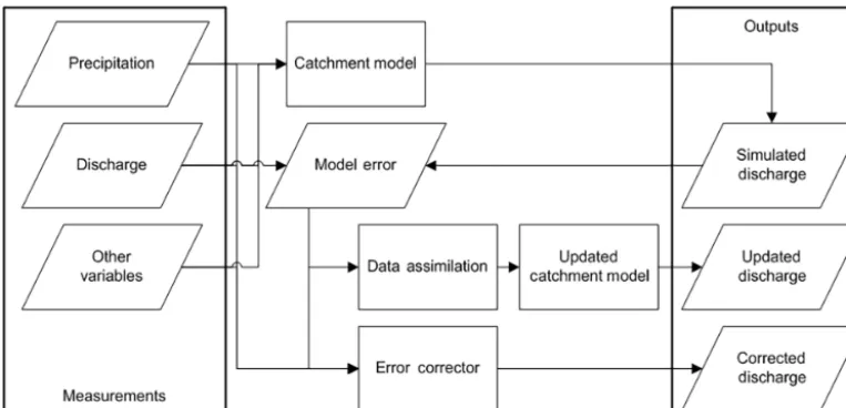
Figure 1.Typical data flow in discharge simulation using hydrological models.
removed from the original network.Relocationis about repo-sitioning the existing network nodes.
The lack of data usually drives the sensor network aug-mentation, whereas economic limitations usually push for re-duction. These costs of the sensor network usually relate to the deployment of physical sensors in the field, and transmis-sion, maintenance, and continuous validation of data (WMO, 2008c).
Augmentation and relocation problems are fundamentally similar, as they require estimation of the measured variable at ungauged locations. For this purpose, statistical models of the measured variable are often employed. For exam-ple, Rodriguez-Iturbe and Mejia (1974) described rainfall regarding its correlation structure in time and space, Pardo-Igúzquiza (1998) expressed areal averages of rainfall events with ordinary Kriging estimation, and Chacon-Hurtado et al. (2009) represented rainfall fields using block Kriging. In contrast, for network reduction, the analysis is driven by what-if scenarios as the measurements become available. Dong et al. (2005) employ this approach to re-evaluate the efficiency of a river basin network based on the results of hydrological modelling.
In principle, augmentation and relocation aim to increase the performance of the network (Pardo-Igúzquiza, 1998; Nowak et al., 2010). In reduction, by contrast, network per-formance is usually decreased. The driver of these decisions is usually related to factors such as operation and mainte-nance costs (Moss et al., 1982; Dong et al., 2005).
1.3 Role of measurements in rainfall–runoff modelling The typical data flow for hydrological rainfall–runoff mod-elling can be summarised as in Fig. 1. For discharge simula-tion, precipitation and evapotranspiration are the most com-mon data requirements (WMO, 2008c; Beven, 2012), while discharge data are commonly employed for model
calibra-tion, correccalibra-tion, and update (Sun et al., 2015). Data-driven hydrological models may use measured discharge as input variables as well (e.g. Solomatine and Xue, 2004; Shrestha and Solomatine, 2006). Methods for updating of hydrologi-cal models have been widely used in discharge forecasting as data assimilation, using the model error to update the model states. In this way, more accurate discharge estimates can be obtained (Liu et al., 2012; Lahoz and Schneider, 2014). In real-time error correction schemes, typically, a data-driven model of the error is employed which may require as input any of the mentioned variables (Xiong and O’Connor, 2002; Solomatine and Ostfeld, 2008).
In a conceptual way, we can express the quantification of discharge at a given station as (Solomatine and Wagener, 2011)
Q= ˆQ (x, θ )+ε, (1)
whereQis the recorded discharge, andQ(x, θ )ˆ represents a hydrological model, which is a function of measured vari-ables (mainly precipitation and discharge,x) and the model parameters (θ).εis the simulation error, which is ideally in-dependent of the model, but in practice is conditioned by it. Considering that neither are the measurements perfect nor the model unbiased, the variance of the estimates is propor-tional to the uncertainty in the model inputs,σ2(x), and the uncertainty in model parameters,σ2(θ ):
σ2Q (x, θ )ˆ ασ2(x) , σ2(θ ) . (2)
2 Classification of approaches for sensor network evaluation
prag-Figure 2. Proposed classification of methods for sensor network evaluation.
matic. In this section, we provide a general classification of these approaches, and more details of each method are given in the next section.
Although most of the approaches for the design of sensor networks make use of data, some rely solely on experience and recommendations. Therefore, a first tier in the proposed classification consists of recognising both measurement-based and measurement-free approaches (Fig. 2). The former make use of the measured data to evaluate the performance of the network (Tarboton et al., 1987; Anctil et al., 2006), while the latter use other data sources (Moss and Tasker, 1991), such as topography and land use.
2.1 Measurement-based evaluation
The measurement-based approach can be further subdivided into model-free and model-based approaches (Fig. 2), de-pending on the use of modelling results in the performance metric.
2.1.1 Model-free performance evaluation
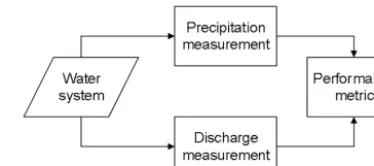
[image:4.612.334.521.66.149.2]In model-free approaches, water systems and the external processes that drive their behaviour are observed through ex-isting measurements, without the use of catchment models. Then, metrics about amount and quality of information in space and time are evaluated with regards to the manage-ment objectives and the decisions to be made in the system. Some performance metrics in this category are joint entropy (Krstanovic and Singh 1992), information transfer (Yang and Burn, 1994), interpolation variance (Pardo-Igúzquiza, 1998; Cheng et al., 2007), and autocorrelation (Moss and Karlinger, 1974), among others. Figure 3 presents the flowchart for the case when precipitation and discharge, as the main drivers of catchment hydrology (WMO, 2008c), are considered in model-free network evaluation.
[image:4.612.81.252.66.244.2]Figure 3.General procedure for model-free sensor network evalua-tion.
Figure 4.General procedure for model-based sensor network eval-uation.
Fundamentally, the model-free approach aims to minimise the variance of the measured variable, thereby (and in theory) minimising the variance in the estimation (Eq. 3). However, a design that is optimal for estimation is not necessarily also optimal for prediction (Chaloner and Verdinelli, 1995).
minσ2Q (x, θ )ˆ αminσ2(x) (3)
Application of model-free approaches can be found in Krstanovic and Singh (1992), Nowak et al. (2010), and Li et al. (2012). Model-free evaluations are suitable for sensor network design aimed mainly at water resource planning, in which diverse water interests must be balanced. Due to the lack of a quantitative performance metric that relates simu-lated discharge, these kinds of evaluations do not necessarily improve rainfall–runoff simulations.
2.1.2 Model-based performance evaluation
In the model-based approach, the performance of sensor net-works is carried out using a catchment model (Dong et al., 2005; Xu et al., 2013). In this case, measurements of precip-itation are used to simulate discharge, which is compared to the discharge measurements at specific locations. Therefore, any metric of the modelling error could be used to evaluate the performance of the network. Figure 4 presents a generic model-based approach for evaluating sensor networks.
[image:4.612.322.537.203.290.2]Therefore, it is possible to identify a set of measurements (x) which minimise the modelling error as
minσ2() αmin
Q− ˆQ (x, θ )
. (4)
The need for the catchment model and possible high com-putational efforts for multiple model runs are some disad-vantages of this approach. The computational load is espe-cially critical in the case of complex distributed models. It is worth mentioning that particular model error metrics (Nash and Sutcliffe, 1970; Gupta et al., 2009) may qualify the net-work by its ability to capture certain hydrological processes (Bennet et al., 2013), affecting the network evaluation. 2.2 Measurement-free evaluation
As is seen from its name, this approach does not require the previous collection of data of the measured variable to eval-uate the sensor network performance. The evaluation of sen-sor networks is based on either experience or physical char-acteristics of the area such as land use, slope, or geology. In this group of methods, the following can be mentioned: case-specific recommendations (Bleasdale, 1965; Wahl and Crippen, 1984; Karasseff, 1986; WMO, 2008a) and physio-graphic components (Tasker, 1986; Laize, 2004). This ap-proach is the first step towards any sensor network develop-ment (Bleasdale, 1965; Moss et al., 1982; Nemec and Askew, 1986; Karasseff, 1986).
3 Classification of methods for sensor network evaluation
In this section, we classify the methods used to quantify the performance of the sensor networks based on the mathe-matical apparatus used to evaluate the network performance. These methods can broadly be categorised as statistics-based, information theory-based, expert recommendations, and oth-ers.
3.1 Statistics-based methods
Statistics-based methods refer to methods where the per-formance of the network is evaluated with statistical un-certainty metrics of the measured or simulated variable. These methods aim to minimise either interpolation vari-ance (Rodriguez-Iturbe and Mejia, 1974; Bastin et al., 1984; Bastin and Gevers, 1985; Pardo-Igúzquiza, 1998; Bonac-corso et al., 2003), cross-correlation (Maddock, 1974; Moss and Karlinger, 1974; Tasker, 1986) or model error (Dong et al., 2005; Xu et al., 2013).
3.1.1 Interpolation variance (geostatistical)
Methods to evaluate sensor networks considering a reduction in the interpolation variance assume that for a network to be
optimal, the measured variable should be as certain as possi-ble in the domain of the propossi-blem. To achieve this, a stochas-tic interpolation model that provides uncertainty metrics is required. Geostatistical methods such as Kriging (Journel and Huijbregts, 1978; Cressie, 1993) or copula interpolation (Bárdossy, 2006) have an explicit estimation of the interpola-tion error. This characteristic makes it suitable for identifying areas with expected poor interpolation results, (Bastin et al., 1984; Pardo-Igúzquiza, 1998; Grimes et al., 1999; Bonac-corso et al., 2003; Cheng et al., 2007; Nowak et al., 2009, 2010; Shafiei et al., 2013).
In the case of Kriging, the optimal estimation of a variable at ungauged locations is assumed to be a linear combination of the measurements, with a Gaussian distributed probabil-ity distribution function. Under the ordinary Kriging formu-lation, the variance in the estimation (σ2)of a variable at location (u)over a catchment is
σ2(u)=C0− n X
α=1
λα(u)−C(uα−u), (5)
whereC0refers to the variance of the random field, andλα are the Kriging weights for the stationαat the ungauged lo-cationu.C (uα−u)is the covariance between the stationα at the locationuα and the interpolation target at the location u.nrepresents the total number of stations in the neighbour-hood ofuand used in the interpolation.
Therefore, as an objective function the optimal sensor net-work is such that the total Kriging variance (TKV) is mini-mum:
TKV=
U X
u=1
σ2(u), (6)
whereU is the total number of discrete interpolation targets in the catchment or domain of the problem.
Bastin and Gevers (1985) optimised a precipitation sen-sor network at pre-defined locations to estimate the average precipitation for a given catchment. Their selection of the op-timal sensor location consisted of minimising the normalised uncertainty by reducing the network. The main drawback of their approach is that the network can only be reduced and not augmented. Similar approaches have also been used by Rodriguez-Iturbe and Mejia (1974), Bogárdi et al. (1985), and Morrissey et al. (1995). Pardo-Igúzquiza (1998) ad-vanced this formulation by removing the pre-defined set of locations (allowing augmentation). Instead, rain gauges were allowed to be placed anywhere in the catchment and its sur-roundings. A simulated annealing algorithm is used to search for the optimal set of sensors to minimise the interpolation uncertainty.
2009). As a geostatistical model, the copula provides met-rics of the interpolation uncertainty, considering not only the location of the stations and the model parameterisation, but also the value of the observations. Li et al. (2011) use the concept of a copula to provide a framework for the design of a monitoring network for groundwater parameter estimation, using a utility function, related to the cost of a given decision with the available information.
In the case of copulas, the full conditional probability dis-tribution function of the variable is interpolated. As such, the interpolation uncertainty depends on the confidence interval, measured values, parameterisation of the copula, and the rel-ative position of the sensors in the domain of the catchment. More details on the formulation of copula-based designs can be found in Bárdossy and Li (2008).
Cheng et al. (2007), as well as Shafiei et al. (2013), recog-nised that the temporal resolution of the measurements af-fects the definition of optimality in minimum interpolation variance methods. This change in the spatial correlation structure occurs due to more correlated precipitation data be-tween stations at coarser sampling resolutions (Ciach and Krajewski, 2006). For this purpose, the sensor network has to be split into two parts, a base network and non-base sen-sors. The former should remain in the same position for long periods, to characterise longer fluctuation phenomena, based on the definition of a minimum threshold for an area with ceptable accuracy. The latter is relocated to improve the ac-curacy of the whole system, and should be relocated as they do not provide a significant contribution to the monitoring objective.
Recent efforts have used minimum interpolation variance approaches to consider the non-stationarity assumption of most geostatistical applications in sensor network design (Chacon-Hurtado et al., 2014). To this end, changes in the precipitation pattern and its effect on the uncertainty esti-mation were considered during the development of a rainfall event.
3.1.2 Cross-correlation
The objective of minimum cross-correlation methods is to avoid placing sensors at sites that may produce redun-dant information. Cross-correlation was suggested by Mad-dock (1974) for sensor network reduction, as a way to iden-tify redundant sensors. In this scope, the objective function can be written as
ρ Xi, Xj= n X
i=1 n X
j=i+1
cov(xi, xj) σ (xi) σ (xj)
, (7)
where cov is the covariance function between a pair of sta-tions (i, j ), andσ is the standard deviation of the observa-tions.
Stedinger and Tasker (1985) introduced the method called network analysis using generalised least squares (NAUGLS), which assesses the parameters of a regression model for
daily discharge simulation based on the physiographic char-acteristics of a catchment (Stedinger and Tasker, 1985; Tasker, 1986; Moss and Tasker, 1991). The method builds a generalised-least-square (GLS) covariance matrix of regres-sion errors to correlate flow records and to consider flow records of different lengths, so the sampling mean squared error can be expressed as
SMSE=1
n j X
i=1
XTi XT3−1X −1
Xi, (8)
whereX[k, w]is the matrix of the (k)basin characteristics in a window of sizew at discharge measuring site i. 3is the GLS weighting matrix, using a set ofngauges (Tasker, 1986).
A comparable method was proposed by Burn and Goul-ter (1991), who used a correlation metric to clusGoul-ter similar stations. Vivekanandan and Jagtap (2012) proposed an alter-native for the location of discharge sensors in a recurrent ap-proach, in which the most redundant stations were removed, and the most informative stations remained using Cooks’D metrics, a measure of how the spatial regression model at a particular site is affected by removing another station. The result of these types of sensors is sparse, as the redundancy of two sensors increases with the inverse of the distance be-tween them (Mishra and Coulibaly, 2009).
3.1.3 Model output error
These methods assume that the optimal sensor network con-figuration is such as satisfies a particular modelling purpose, e.g. a minimum error in simulated discharge. Considering this, the design of a sensor network should be such as min-imises the difference between the simulated and recorded variables:
minf
Q− ˆQ (x, θ )
, (9)
wheref is a metric that summarises the vector error such as bias, root mean squared error (RMSE), or Nash–Sutcliffe efficiency (NSE);Qare the measurements of the simulated variable, andQˆ are the simulation results using inputsx and parametersθ. Bias measures the mean deviation of the results between the observations (Q)and simulation results (Q) forˆ tpairs of observations and simulation results:
Bias=1
n t X
i=1
ˆ
Qi−Qi
. (10)
This metric theoretically varies from minus infinity to infin-ity, and its optimal value is equal to 0. The RMSE measures the standard deviation of the residuals as
RMSE=
v u u t 1 n
t X
i=1
ˆ
Qi−Qi 2
The RMSE can then vary from 0 to infinity, where 0 repre-sents a perfect fit between model results and observations. As RMSE is a statistical moment of the residuals, the result is a magnitude rather than a score. Therefore, benchmark-ing between different case studies is not trivial. To overcome this issue, Nash and Sutcliffe (1970) proposed a score (also known as the coefficient of determination) based on the ratio of the model results in variance over the observation variance as
NSE=1−
t P
i=1
ˆ
Qi−Qi 2
t P
i=1
Qi−Qi 2
, (12)
in whichQare the measurements,Qˆ are the model results, andQis the average of the recorded series.
Theoretically, this score varies from minus infinity to 1. However, its practical range lies between 0 and 1. On the one hand, an NSE equal to 0 indicates that the model has the same explanatory capabilities as the mean of the observations. On the other end, a value of 1 represents a perfect fit between model results and observations. Model output error formula-tions have been used to identify the most convenient set of sensors that provide the best model performance (Tarboton et al., 1987) to propose measurement strategies regarding the number of gauges and sampling frequency.
Another application is provided by Dong et al. (2005), who proposed evaluating the rainfall network using a lumped HBV model (Lindström et al., 1997). They found that the model performance does not necessarily improve when ex-tra rain gauges are placed. A similar approach was presented by Xu et al. (2013), who evaluated the effect of diverse rain gauge locations on runoff simulation using a similar hydro-logical model. It was found that rain gauge locations could have a significant impact and suggests that a gauge density of less than 0.4 stations per 1000 km2can negatively affect the model performance.
Anctil et al. (2006) aimed at improving lumped neural net-work rainfall–runoff forecasting models through mean areal rainfall optimisation, and concluded that different combina-tions of sensors lead to noticeable streamflow forecasting improvements. Studies in other fields have also used this method. For example, Melles et al. (2009, 2011) obtained op-timal monitoring designs for radiation monitoring networks, which minimise the prediction error of mean annual back-ground radiation. The main drawback of this approach is that multiple error metrics are considered, as specific objectives relate to different processes.
3.2 Information-theory-based methods
The use of information theory (Shannon, 1948) in the design of sensor networks for environmental monitoring is based on communication theory, which studies the problem of trans-mitting signals from a source to a receiver throughout a
noisy medium. Information theory provides the possibility of estimating probability distribution functions in the pres-ence of partial information with the less biased estimation (Jaynes, 1957). Some of its concepts are analogous to statis-tics concepts, and therefore similarities between entropy and uncertainty, such as mutual information and correlation, can be found (Cover and Thomas, 2005; Alfonso, 2010; Singh, 2013).
Information theory-based methods for designing sensor networks mainly consider the maximisation of information content that sensors can provide, in combination with the minimisation of redundancy among them (Krstanovic and Singh, 1992; Mogheir and Singh, 2002; Alfonso et al., 2010a, b, 2013; Alfonso, 2010; Singh, 2013). Redundancy can be measured by using mutual information (Singh, 2000; Steuer et al., 2002), directional information transfer (Yang and Burn, 1994), or total correlation (Alfonso et al., 2010a, b; Fahle et al., 2015), among others.
3.2.1 Entropy
The principle of maximum entropy (POME) is based on the premise that probability distribution with the largest remain-ing uncertainty (i.e. the maximum entropy) is the one that best represents the current stage of knowledge. POME has been used as a criterion for the design of sensor networks, by allowing the identification of the set of sensors that max-imises the joint entropy among measurements (Krstanovic and Singh, 1992), in other words, to provide as much infor-mation content, from the inforinfor-mation theory perspective, as possible (Jaynes, 1988).
In the design of sensor networks, the objective is to max-imise the joint entropy (H )of the sensor network as
H (X1, X2, . . ., Xn)= − k X
i=1 . . .
m X
j=1
p xi1, . . .xj m
logp xi1, . . .xj m, (13) wherep(X)is the probability of the random variableX tak-ing a discrete valuexm. As in many applications,Xis a con-tinuous variable which has to be discretised (quantised) into intervals (k,m)to calculate its entropy. The probabilities are calculated following frequency analysis, such that the proba-bility of a variableXtaking a value in the intervali, . . . ,j is defined by the number of times in which this value appears, divided by the complete length of the dataset. When calcu-lating the entropy of more than one variable simultaneously (joint entropy), joint probabilities are used.
network (in the case of high redundancy) or to expand it (in the case of a lack of common information).
Fuentes et al. (2007) proposed an entropy-utility crite-rion for environmental sampling, particularly suited for air-pollution monitoring. This approach considers Bayesian op-timal sub-networks using an entropy framework, relying on the spatial correlation model. An interesting contribution of this work is the assumption of non-stationarity, contrary to traditional atmospheric studies, and relevant in the design of precipitation sensor networks.
Hydraulic 1-D models and metrics of entropy have been used to select the adequate spacing between sensors for wa-ter level in canals and polder systems (Alfonso et al., 2010a, b). This approach is based on the current conditions of the system, which makes it useful for operational purposes, but it does not necessarily support the modifications in the water system conditions or changes in the operation rules. Studies on the design of sensor networks using these methods have been on the rise in recent years (Alfonso, 2010; Alfonso et al., 2013; Ridolfi et al., 2014; Banik et al., 2017).
Benefits of POME include the robustness of the descrip-tion of the posterior probability distribudescrip-tion since it aims to define the less biassed outcome. This is because neither the models nor the measurements are completely certain. Li et al. (2012) presented, as part of a multi-objective framework for sensor network optimisation, the criteria of maximum (joint) entropy, as one of the objectives. Other studies in this direction have been presented by Lindley (1956), Caselton and Zidek (1984), Guttorp et al. (1993), Zidek et al. (2000), Yeh et al. (2011), and Kang et al. (2014).
More recently, Samuel et al. (2013) and Coulibaly and Samuel (2014) proposed a mixed method involving re-gionalisation and dual entropy multi-objective optimisation (CRDEMO), which is a step forward when compared to single-objective optimisation for sensor network design. 3.2.2 Mutual information (trans-information)
Mutual information is a measurement of the amount of infor-mation that a variable contains about another. This is mea-sured as the relative entropy between the joint distribution and the product distribution(Cover and Thomas, 2005). In the simplest expression (two variables), the mutual informa-tion can be defined as
I (X1, X2)=H (X1)+H (X2)−H (X1, X2) , (14) whereH (X1)andH (X2)is the entropy of each of the vari-ables, andH (X1, X2)is the joint entropy between them. The extension of the mutual information for more than two vari-ables should not only consider the joint entropy between them, but also the joint entropy between pairs of variables, leading to a significantly complex expression for the variate mutual information. Regarding this issue, the multi-variate mutual information can be addressed as a nested
prob-lem, such that
I (X1, X2, . . ., Xn)=I (X1, X2, . . ., Xn−1)
−I (X1, X2, . . ., Xn−1|Xn) , (15) whereI (X1, X2, . . . ,Xn)is the multivariate mutual informa-tion among n variables, andI (X1, X2, . . . ,Xn−1|Xn)is the conditional information ofn−1 variables with respect to the nth variable. The conditional mutual information can be un-derstood as the amount of information that a set of variable share with another variable (or variables). The conditional mutual information of two variables (X1 andX2)with re-spect to a third one (X3)can be quantified as
I (X1, X2|X3)=H (X1|X3)−H (X1|X2, X3) , (16) whereH (X1|X3)is the conditional entropy ofX1toX3and H (X1|X2,X3)is the conditional entropy ofX1with respect toX2 andX3 simultaneously. The conditional entropy can be understood as the amount of information that a variable does not share with another. The joint entropy between two variables can be quantified as
H (X1|X2)= k X
i=1 m X
j=1
p X1i, X2j
log p (X1i) p X1i, X2j
, (17)
wherep(X1, X2)is the joint probability, forkandmdiscrete values, ofX1andX2.
An optimal sensor network should avoid collecting repeti-tive or redundant information; in other words, it should re-duce the mutual (shared) information between sensors in the network. Alternatively, it should maximise the trans-ferred information from a measured to a modelled variable at a point of interest (Amorocho and Espildora, 1973). Fol-lowing this idea, Husain (1987) suggested an optimisation scheme for the reduction of a rain sensor network. His objec-tive was to minimise the trans-information between pairs of stations. However, assumptions of the probability and joint probability distribution functions are strong simplifications of this method. To overcome these assumptions, the Di-rectional Information Transfer (DIT) index was introduced (Yang and Burn, 1994) as the inverse of the coefficient of non-transferred information (NTI) (Harmancioglu and Yev-jevich, 1985). Both DIT and NTI are a normalised measure of information transfer between two variables (X1andX2). DIT=I (X1, X2)
H (X1)
Total correlation (C) is an alternative measure of the amount of shared information between two or more vari-ables, and has also been used as a measure of information redundancy in the design of sensor networks (Alfonso et al., 2010a, b; Leach et al., 2015) as
C (X1, . . ., Xn)= n X
i=1
H (Xi)−H (X1, . . ., XN), (19)
where C(X1, X2, . . . , Xn) is the total correlation among the nvariables,H (Xi)is the entropy of the variablei, and H (X1, X2, . . . ,Xn)is the joint entropy of then variables. Total correlation can be seen then as a simplification of the multivariate mutual information, where only the interaction among all the variables is considered. In the design of sensor networks, it is expected that the mutual information among the different variables is minimum; therefore, the difference between the total correlation and multivariate mutual infor-mation tends to be minimised as well. The advantage of total correlation is the computational advantage that represents as-suming a marginal value for the interaction among variables. A method to estimate trans-information fields at ungauged locations has been proposed by Su and You (2014), employ-ing a trans-information–distance relationship. This method accounts for spatial distribution of precipitation, supporting the augmentation problem in the design of precipitation sen-sor networks. However, as the relationship between trans-information between sensors and their distance is monotonic, the resulting sensor networks are generally sparse.
3.3 Methods based on expert recommendations 3.3.1 Physiographic components
Among the most used planning tools for hydrometric net-work design are the technical reports presented by the WMO (2008c), in which a minimum density of stations de-pending on different physiographic units, are suggested (Ta-ble 1). Although these guidelines do not provide an indica-tion about where to place hydrometric sensors, rather they recommend that their distribution should be as uniform as possible and that network expansion has to be considered. The document also encourages the use of computationally aided design and evaluation of a more comprehensive de-sign. For instance, Coulibaly et al. (2013) suggested the use of these guidelines to evaluate the Canadian national hydro-metric network.
Moss et al. (1982) presented one of the first attempts to use physiographic components in the design of sensor networks in a method called Network Analysis for Regional Informa-tion (NARI). This method is based on relaInforma-tions of basin char-acteristics proposed by Benson and Matalas (1967). NARI can be used to formulate the following objectives for network design: minimum cost network, maximum information, and maximum net benefit from the data-collection programme, in
a Bayesian framework, which can be approximated as
logσS
ˆ
Q−Q
α
=a+ b1
n + b2
y, (20)
where the functionS(| ˆQ−Q|)α is the α percentile of the standard error in the estimation ofQ,a,b1, andb2are the pa-rameters from the NARI analysis,nis the number of stations used in the regional analysis, andy is the harmonic mean of the records used in the regression.
Laize (2004) presented an alternative for evaluating pre-cipitation networks based on the use of the Representative Catchment Index (RCI), a measure to estimate how repre-sentative a given station in a catchment is for a given area, on the stations in the surrounding catchments. The author argues that the method, which uses datasets of land use and eleva-tion as physiographical components, can help in identifying areas with an insufficient number of representative stations in a catchment.
3.3.2 Practical case-specific considerations
Most of the first sensor networks were designed based on ex-pert judgement and practical considerations. Aspects such as the objective of the measurement, security, and accessibility are decisive to selecting the location of a sensor. Nemec and Askew (1986) presented a short review of the history and development of the early sensor networks, where it is high-lighted that the use of “basic pragmatic approaches” still had most of the attention, due to its practicality in the field and its closeness with decision-makers.
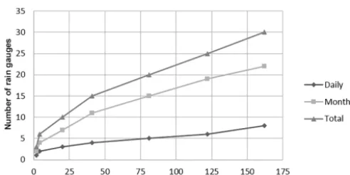
Bleasdale (1965) presented a historical review of the early development process of the rainfall sensor networks in the United Kingdom. In the early stages of the development of precipitation sensor networks, two main characteristics influ-encing the location of the sensors were identified: at sites that were conventionally satisfactory and where good observers were located. However, the necessity of a more structured approach to select the location of sensors was underlined. As a guide, Bleasdale (1965) presented a series of recommenda-tions on the minimal density of sensors for operational pur-poses, summarised in Fig. 5, relating the characteristics of the area to be monitored and the minimum required a num-ber of rain sensors, as well as its temporal resolution.
In a more structured approach, Karasseff (1986) intro-duced some guidelines for the definition of the optimal sen-sor network to measure hydrological variables for opera-tional hydrological forecasting systems. The study specified the minimum requirements for the density of measurement stations based on the fluctuation scale and the variability of the measured variable by defining zonal representative areas. This author suggested the following considerations for se-lecting the optimal placement of hydrometric stations:
Table 1.Recommended minimum densities of stations (area in km2per station) – adapted from WMO (2008c).
Precipitation
Physiographic unit Non-recording Recording Evaporation Streamflow Sediments Water quality
Coastal 900 9000 50 000 2750 18 300 55 000
Mountains 250 2500 50 000 1000 6700 20 000
Interior plains 575 5750 5000 1875 12 500 37 500
Hilly/undulating 575 5750 50 000 1875 12 500 47 500
Small islands 25 250 50 000 300 2000 6000
Urban areas – 10–20 – – – –
Polar/arid 10 000 10 000 100 000 20 000 200 000 200 000
Figure 5.Minimum number of rain gauges required in reservoired moorland areas – adapted from Bleasdale (1965).
– at the heads of irrigation and watering canals taking wa-ter from the sources;
– at the beginning of a debris cone before the zone of in-filtration, and at its end, where groundwater decrement takes place;
– at the boundaries of irrigated areas and zones of consid-erable industrial water diversions (towns); and
– at the sites of hydroelectric power plants and hydro-projects.
From a different perspective, Wahl and Crippen (1984), as well as Mades and Oberg (1986), proposed a qualitative score assessment of different factors related to the use of data and the historical availability of records for the evaluation of sor values. Their analyses aimed at identifying candidate sen-sors to be discontinued, due to their limited accuracy. 3.3.3 User survey
These approaches aim to identify the information needs of particular groups of users (Sieber, 1970), following the idea that the location of a certain sensor (or group of sensors) should satisfy at least one specific purpose. To this end, sur-veys to identify the interests for the measurement of cer-tain variables, considering the location of the sensor, record
length, frequency of the records, methods of transmission, among others, are executed.
Singh et al. (1986) applied two questionnaires to evalu-ate the streamflow network in Illinois: one to identify the main uses of streamflow data collected at gauging stations, where participants described how data was used and how they would categorise it in either site-specific management activities, local or regional planning and design, or deter-mination of long-term trends. The second questionnaire was used to determine present and future needs for streamflow information. The results showed that the network was re-duced due to the limited interest about certain sensors, which allowed for enhancing the existing network using more so-phisticated sensors or recording methods. Additionally, this redirection of resources increased the coverage at specific lo-cations.
3.4 Other methods
There are also other methods that cannot be easily attributed to the previously mentioned categories. Among them, value of information, fractal, and network theory-based methods can be mentioned.
3.4.1 Value of information
The value of information (VOI, Howard, 1966; Hirshleifer and Riley, 1979) is defined as the value a decision-maker is willing to pay for extra information before making a deci-sion. This willingness to pay is related to the reduction of uncertainty about the consequences of making a wrong deci-sion (Alfonso and Price, 2012).
[image:10.612.45.291.231.354.2]One of the assumptions of this type of model is that a prior estimation of consequences is needed. Ifa is the action that has been decided to perform,mis the additional information that comes to make such a decision, andsis the state that is actually observed, then the expected utility of any action a can be expressed as
u (a, Ps)= X
S
Psu (Cas) , (21)
wherePs is the perception, in probabilistic terms, of the oc-currence of a particular state (s)among a total number of pos-sible states (S), anduis the utility of the outcomeCasof the actions given the different states. When new information (i.e. a messagem)becomes available, and the decision-maker ac-cepts it, his prior beliefPs will be subject to a Bayesian up-date. IfP (m|s)is the likelihood of receiving the messagem given the statesandPmis the probability of getting a mes-sagem, then
Pm= X
S
PsP (m|s) . (22)
The value of a single messagemcan be estimated as the difference between the utility,u, of the action,amthat is cho-sen given a particular messagemand the utility of the action, a0, that would have been chosen without additional informa-tion as
1m=u (am, P (s|m))−u (a0, P (s|m)) . (23) The value of information, VOI, is the expected utility of the values1m:
VOI=E (1m)= X
M
Pm1m. (24)
Following the same line of ideas, Khader et al. (2013) proposed the use of decision trees to account for the de-velopment of a sensor network for water quality in drinking groundwater applications. VOI is a straightforward method-ology to establish present causes and consequences of sce-narios with different types of actions, including the expected effect of additional information. A recent effort by Alfonso et al. (2016) towards identifying valuable areas to get informa-tion for floodplain planning consists of the generainforma-tion of VOI maps, where probabilistic flood maps and the consequences of urbanisation actions are taken into account to identify ar-eas where extra information may be more critical.
3.4.2 Fractal-based
Fractal-based methods employ the concept of Gaussian self-affinity, where sensor networks show the same spatial pat-terns at different scales. This affinity can be measured by its fractal dimension (Mandelbrot, 2001). Lovejoy et al. (1986)
proposed the use of fractal-based methods to measure the di-mensional deficit between the observations of a process and its real domain. Consider a set of evenly distributed cells rep-resenting the physical space, and the fractal dimension of the network representing the number of observed cells in the cor-relation space. The lack of non-measured cells in the corre-lation space is known as the fractal deficit of the network. Considering that a large number of stations have to be avail-able at different scales, the method is suitavail-able for large net-works, but less useful in the deployment of few sensors in a catchment scale.
Lovejoy and Mandelbrot (1985) and Lovejoy and Schertzer (1985) introduced the use of fractals to model pre-cipitation. They argued that the intermittent nature of the at-mosphere can be characterised by fractal measures with fat-tailed probability distributions of the fluctuations, and stated that standard statistical methods are inappropriate to describe this kind of variability. Mazzarella and Tranfaglia (2000) and Capecchi et al. (2012) presented two different case studies using this method for the evaluation of a rainfall sensor net-works. The former study concludes that for network augmen-tation, it is important to select the optimal locations that im-prove the coverage, measured by the reduction of the fractal deficit. However, there are no practical recommendations on how to select such locations. The latter proposes the inspec-tion of seasonal trends as the meteorological processes of precipitation may have significant effects on the detectabil-ity capabilities of the network.
A common approach for the quantification of the dimen-sional deficit is the box-counting method (Song et al., 2007; Kanevski, 2008), mainly used in the fractal characterisation of precipitation sensor networks. The fractal dimension of the network (D)is quantified as the ratio of the logarithm of the number of blocks (NB) that have measurements and the logarithm of the scaling radius (R).
D= log(NB(R))
log(R) (25)
Due to the scarcity of measurements of precipitation types of networks, the quantification of the fractal dimension may be unstable. An alternative fractal dimension may be calcu-lated using a correlation integral (Mazzarella and Tranfaglia, 2000) instead of the number of blocks, such that
CI(R)= 2
B(B−1) B X
i=1 B X
j=1
2 R−uαi−uαj
:
for i6=j, (26)
The consequent definition of the fractal dimension of the network is the rate between the logarithm of the correlation integral and the logarithm of the scaling radius. This ratio is calculated from a regression between different values ofR, for which the network exhibits fractal behaviour (meaning a high correlation between log(CI) and log(R)).
D=log(CI)
log(R) (27)
The maximum potential value for the fractal dimension of a 2-D network (such as for spatially distributed variables) is 2. However, this limit considers that the stations are located on a flat surface, as elevation is a consequence of the topography, and is not a variable that can be controlled in the network deployment.
3.4.3 Network theory-based
Recently, research efforts have been devoted to the use of the so-called network theory to assess the performance of dis-charge sensor networks (Sivakumar and Woldemeskel, 2014; Halverson and Fleming, 2015). These studies analyse three main features, namely average clustering coefficient, average path length, and degree distribution. Average clustering is a degree of the tendency of stations to form clusters. Average path length is the average of the shortest paths between every combination of station pairs. Degree distribution is the prob-ability distribution of network degrees across all the stations, being network degree defined as the number of stations to which a station is connected. Halverson and Fleming (2015) observed that regular streamflow networks are highly clus-tered (so the removal of any randomly chosen node has little impact on the network performance) and have long average path lengths (so information may not easily be propagated across the network).
In hydrometric networks, three metrics are identified (Halverson and Fleming, 2015): degree distribution, cluster-ing coefficient, and average path length. The first of these measures is the average node degree, which corresponds to the probability of a node being connected to other nodes. The metric is calculated in the adjacency matrix (a binary matrix in which connected nodes are represented by 1 and the miss-ing links by 0). Therefore, the degree of the node is defined as
k(α)=
n X
j=1
aα,j, (28)
wherek(α)is the degree of stationα,nis the total number of stations, andais the adjacency matrix.
The clustering coefficient is a measure of how much the nodes cluster together. High clustering indicates that nodes are highly interconnected. The clustering coefficient (CC) for
a given station is defined as
CC(α)= 2
k (α) (k (α)−1) n X
j=1
aα,j. (29)
Additionally, the average path length refers to the mean dis-tance of the interconnected nodes. The length of the connec-tions in the network provides some insights into the length of the relationships between the nodes in the network.
L= 1
n(n−1) k(α) X
α=1 n X
j=1
dα,j (30)
As can be seen from the formulation, the metrics of the net-work largely depend on the definition of the netnet-work topol-ogy (adjacency matrix). The links are defined from a metric of statistical similitude such as the Pearsonr or the Spear-man rank coefficient. The links are such a pair of stations over which statistical similitude is over a certain threshold.
According to Halverson and Fleming (2015), an opti-mal configuration of streamflow networks should consist of measurements with small membership communities, high-betweenness, and index stations with large numbers of in-tracommunity links. Small communities represent clusters of observations, thus indicating efficient measurements. Large numbers of intra-community links ensure that the network has some degree of redundancy, and, thus, is resistant to sensor failure. High-betweenness indicates that such stations which have the most inter-communal links are adequately connected and thus able to capture the heterogeneity of the hydrological processes at a larger scale.
3.5 Aggregation of approaches and classes
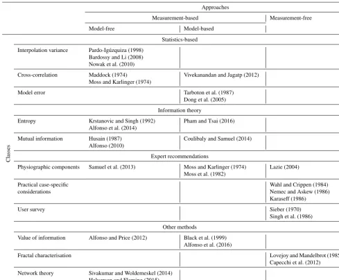
Table 2 summarises the sensor network design classes and approaches, with the selected references to the relevant pa-pers in each of the categories for further reference.
It is of special interest in the review to highlight the lack of model-based information theory methods, as well as the low number of publications in network theory-based meth-ods. Also, quantitative studies in the comparison of different methodologies for the design of sensor networks are limited. It is suggested, therefore, that a pilot catchment is used for the scientific community to test all the available methods for network evaluation, and to establish similarities and differ-ences among them.
Table 2.Classification of sensor network design criteria including recommended reading.
Approaches
Measurement-based Measurement-free
Model-free Model-based
Classes
Statistics-based
Interpolation variance Pardo-Igúzquiza (1998) Bardossy and Li (2008) Nowak et al. (2010)
Cross-correlation Maddock (1974) Vivekanandan and Jagatp (2012) Moss and Karlinger (1974)
Model error Tarboton et al. (1987) Dong et al. (2005)
Information theory
Entropy Krstanovic and Singh (1992) Pham and Tsai (2016) Alfonso et al. (2014)
Mutual information Husain (1987) Coulibaly and Samuel (2014) Alfonso (2010)
Expert recommendations
Physiographic components Samuel et al. (2013) Moss and Karlinger (1974) Lazie (2004) Moss et al. (1982)
Practical case-specific Wahl and Crippen (1984) considerations Nemec and Askew (1986)
Karaseff (1986)
User survey Sieber (1970) Singh et al. (1986)
Other methods
Value of information Alfonso and Price (2012) Black et al. (1999) Alfonso et al. (2016)
Fractal characterisation Lovejoy and Mandelbrot (1985) Capecchi et al. (2012)
Network theory Sivakumar and Woldemeskel (2014) Halverson and Fleming (2015)
4 General procedure for sensor network design
Based on the presented literature review, in this section an attempt is made to present a first version of a unified, gen-eral procedure for sensor network design. Such procedure logically link in a flowchart various methods, following the measurement-based approaches (Fig. 6). The flowchart sug-gests two main loops: one to measure the network perfor-mance (optimisation loop), and a second one to represent the selection in the number of sensors in either augmenta-tion or reducaugmenta-tion scenarios. Most of the measurement-based methods, as well as most of the design scenarios can be typ-ically seen as particular cases of this generalised algorithmic flowchart.
The general procedure consists of 11 steps (boxes in Fig. 6). In the first place, physical measurements (1) are ac-quired by the sensor network. These data are used to param-eterise an estimator (2), which will be used to estimate the
variable at the candidate measurement locations (CML) us-ing, for instance, Kriging (Pardo-Igúzquiza, 1998; Nowak et al., 2009) or 1-D hydrodynamic models (Neal et al., 2012; Rafiee, 2012; Mazzoleni et al., 2015). The sensor network reduction does not require such estimators as measurements are already in place.
The selection of the CML should consider factors such as physical and technical availability, as well as costs related to maintenance and accessibility of stations, as illustrated by the WMO (2008c) recommendations. The selection of CML can also be based, for example, on expert judgement. These limitations may be presented in the form of constraints in the optimisation problem.
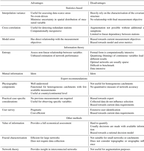
dis-Table 3.Advantages and disadvantages of sensor network design methods.
Advantages Disadvantages
Statistics-based
Interpolation variance Useful for assessing data-scarce areas No event-driven
Heavily rely on the characterisation of the covariance structure
Minimise uncertainty in spatial distribution of mea-sured variable
No relationship with final measurement objective
Cross-correlation Useful for detecting redundant stations Computationally inexpensive
Augmentation not possible without additional as-sumptions
Limited to linear dependency between stations
Model error Has direct relationship with the measurement Biased towards current measurement objectives
objectives Biased towards model and error metrics
Information theory
Entropy Assess non-linear relationship between variables Formal form is computationally intensive
Unbiased estimation of network performance Quantising (binning) of continuous variables lead to different results
Optimal networks are usually sparse Difficult to benchmark
Data intensive
Mutual information Idem Idem
Expert recommendations
Physiographic Well understood Not useful for homogeneous catchments
components Functional for heterogeneous catchments with few available measurements
No quantitative measure of network accuracy
Useful at country/continental level
Practical case-specific No previous measurements are required Biased towards expert
considerations Useful for observing specific variables Collected data do not influence selection Biased towards current data requirements
User survey Pragmatic Extensive user identification
Cost-efficient Biased towards current data requirements
Other methods
Value of information Provides a full economical assessment Hard to quantify
Usually decisions are made with available informa-tion
Biased towards a rational decision model
Fractal characterisation Efficient for large networks Not suitable for small networks or catchments Does not require data collection Does not consider topographic or orographic
influ-ence
Network theory Provides insight in interconnected networks Not useful for augmentation purposes Data intensive
cussed methods. The selection of the method depends on the designer and its information requirements, which also deter-mine whether an optimal solution is found (5). The stopping criteria in the optimisation problem can be set by a desired accuracy of the network, some non-improved number of so-lutions, or a maximum number of iterations. As pointed out in the review, these performance metrics can be either
model-based or model-free and should not be confused with the use of a (geostatistical) model of the measured variable.
[image:14.612.47.550.86.613.2]ex-Figure 6. Sensor network (re)design flowchart (CML: candidate measurement locations).
pected performance of the network, but also recognise the effect of a limited number of sensors.
Once the performance is optimal, an iteration over the number of sensors is required. If the scenario is for network augmentation (7), then a possibility of including additional sensors has to be considered (8). The decision to go for an additional sensor will depend on the constraints of the prob-lem, such as a limitation on the number of sensors to install, or on the marginal improvement of performance metrics.
The network reduction scenario (9) is inverse: for diverse reasons, mainly of a financial nature, networks require fewer sensors. Therefore, the analysis concerns which sensors to re-move from the network, within the problem constraints (10). Finally, the sensor network is selected (11) from the re-sults of the optimisation loop, with the adequate number of
sensors. It is worth mentioning that an extra loop is required, leading to re-evaluation, typically done on a periodical basis, when objectives of the network may be redefined, new pro-cesses need to be monitored, or when information from other sources is available, and that can potentially modify the def-inition of optimality.
5 Conclusions and recommendations
This paper summarised some of the methodological criteria for the design of sensor networks in the context of hydro-logical modelling, proposed a framework for classifying the approaches in the existing literature, and also proposed a gen-eral procedure for sensor network design. The following con-clusions can be drawn.
Most of the sensor network methodologies aim to min-imise the uncertainty of the variable of interest at ungauged locations and the way this uncertainty is estimated varies be-tween different methods. In statistics-based models, the ob-jective is usually to minimise the overall uncertainty about precipitation fields or discharge modelling error. Informa-tion theory-based methods aim to find measurements at loca-tions with maximum information content and minimum re-dundancy. In network theory-based methods, estimations are generally not accurate, resulting in less biassed estimations. In methods based on practical case-specific considerations and value of information, the critical consequences of deci-sions dictate the network configuration.
However, in spite of the underlying resemblances between methods, different formulations of the design problem can lead to rather different solutions. This gap between methods has not been deeply covered in the literature and therefore general agreement on the sensor network design procedure is relevant.
In particular, for catchment modelling, the driving criteria should also consider model performance. This driving crite-rion ensures that the model adequately represents the states and processes of the catchment, reducing model uncertainty and leading to more informed decisions. Currently, most of the network design methods do not ensure minimum mod-elling error, as often it is not the main performance criteria for design.
[image:15.612.82.252.64.475.2]re-ducing limitations of various sensing techniques, and at the same time require the new network design methods allowing for handling of the heterogeneous dynamic data with varying uncertainty.
The proposed classification of the available network de-sign methods was used to develop a general framework for network design. Different design scenarios, namely reloca-tion, augmentareloca-tion, and reduction of networks, are included for measurement-based methods. This framework is open and offers “placeholders” for various methods to be used de-pending on the problem type.
Concerning the further research, from the hydrological modelling perspective, we propose directing efforts towards the joint design of precipitation and discharge sensor net-works. Hydrological models use precipitation data to provide discharge estimates; however, as these simulations are error-prone, the assimilation of discharge data, or error correction, reduces the systematic errors in the model results. The joint design of both precipitation and discharge sensor networks may help to provide more reliable estimates of discharge at specific locations.
Another direction of research may include methods for designing dynamic sensor networks, given the increasing availability of low-cost sensors, as well as the expansion of citizen-based data collection initiatives (crowdsourcing). These information sources have been on the rise in recent years, and one may foresee the appearance of interconnected, multi-sensor heterogeneous sensor networks shortly.
The presented review has also shown that limited effort has been devoted to considering changes in long-term patterns of the measured variable in the sensor network design. This as-sumption of stationarity has become more relevant in recent years due to new sensing technologies and increased sys-temic uncertainties, e.g. due to climate and land use change and rapidly changing weather patterns. Although this topic has been recognised for quite some time already (see e.g. Nemec and Askew, 1986), the number of publications pre-senting effective methods to deal with them is still limited. This problem, and the techniques to solve it, are being ad-dressed in the ongoing research.
Data availability. No data sets were used in this article.
Competing interests. The authors declare that they have no conflict of interest.
Acknowledgements. We would like to thank Joanne Craven for the editing support in the final stages of this article, and the three anonymous referees whose comments greatly helped us to improve this document to its current form.
Edited by: Laurent Pfister
Reviewed by: three anonymous referees
References
Alfonso, L.: Optimisation of monitoring networks for water sys-tems Information theory, value of information and public partici-pation, PhD thesis, UNESCO-IHE and Delft University of Tech-nology, CRC-Press, Delft, the Netherlands, 2010.
Alfonso, L. and Price, R.: Coupling hydrodynamic mod-els and value of information for designing stage mon-itoring networks, Water Resour. Res., 48, W08530, https://doi.org/10.1029/2012WR012040, 2012.
Alfonso, L., Lobbrecht, A., and Price, R.: Optimization of Water Level Monitoring Network in Polder Systems Us-ing Information Theory, Water Resour. Res., 46, W12553, https://doi.org/10.1029/2009WR008953, 2010a.
Alfonso, L., Lobbrecht, A., and Price, R.: Information theory–based approach for location of monitoring water level gauges in polders, Water Resour. Res., 46, W12553, https://doi.org/10.1029/2009WR008101, 2010b.
Alfonso, L., He, L., Lobbrecht, A., and Price, R.: Informa-tion theory applied to evaluate the discharge monitoring net-work of the Magdalena River, J. Hydroinform., 15, 211–228, https://doi.org/10.2166/hydro.2012.066, 2013.
Alfonso, L., Ridolfi, E., Gaytan-Aguilar, S., Napolitano, F., and Russo, F.: Ensemble entropy for monitoring network design, En-tropy, 16, 1365–1375, https://doi.org/10.3390/e16031365, 2014. Alfonso, L., Chacon-Hurtado, J., and Peña-Castellanos, G.: Allow-ing citizens to effortlessly become rainfall sensors, 36th IAHR World Congress, the Hague, the Netherlands, 2015.
Alfonso, L., Mukolwe, M., and Di Baldassarre, G.: Proba-bilistic flood maps to support decision-making: Mapping the Value of Information, Water Resour. Res., 52, 1026–1043, https://doi.org/10.1002/2015WR017378, 2016.
Amorocho, J. and Espildora, B.: Entropy in the assessment of uncer-tainty in hydrologic systems and models, Water Resour. Res., 9, 1511–1522, https://doi.org/10.1029/WR009i006p01511, 1973. Anctil, F., Lauzon, N., Andréassian, V., Oudin, L., and
Per-rin, C.: Improvement of rainfall-runoff forecast through mean areal rainfall optimization, J. Hydrol., 328, 717–725, https://doi.org/10.1016/j.jhydrol.2006.01.016, 2006.
Ballari, D., de Bruin, S., and Bregt, A. K.: Value of information and mobility constraints for sampling with mobile sensors, Comput. Geosci., 49, 102–111, https://doi.org/10.1016/j.cageo.2012.07.005, 2012.
Banik, B. K., Alfonso, L., Di Cristo, C., Leopardi, A., and Mynett, A.: Evaluation of different formulations to optimally locate pollution sensors in sewer systems, ASCE J. Water Res. Pl., https://doi.org/10.1061/(ASCE)WR.1943-5452.0000778, 2017. Barca, E., Pasarella, G., Vurro, M., and Morea, A.: MSANOS:
Data-Driven, Multi-Approach Software for Optimal Redesign of En-vironmental Monitoring Networks, Water Resour. Manag., 29, 619–644, https://doi.org/10.1007/s11269-014-0859-9, 2015. Bárdossy, A.: Copula-based geostatistical models for
Bárdossy, A. and Li, J.: Geostatistical interpolation using copulas, Water Resour. Res., 44, W07412, https://doi.org/10.1029/2007WR006115, 2008.
Bárdossy, A. and Pegram, G. G. S.: Copula based multisite model for daily precipitation simulation, Hydrol. Earth Syst. Sci., 13, 2299–2314, https://doi.org/10.5194/hess-13-2299-2009, 2009. Bastin, G. and Gevers, M.: Identification and optimal estimation
of random fields from scattered point-wise data, Automatica, 2, 139–155, https://doi.org/10.1016/0005-1098(85)90109-8, 1985. Bastin, G., Lorent, B., Duque, C., and Gevers, M.: Optimal
es-timation of the average areal rainfall and optimal selection of rain gauge locations, Water Resour. Res., 20, 463–470, https://doi.org/10.1016/0005-1098(85)90109-8, 1984.
Bennet, N. D., Croke, B. F. W., Guariso, G., Guillaume, J. H., Hamilton, S. H., Jakeman, A. J., Marsili-Libelli, S., Newham, L. T. H., Norton, J. P., Perrin, C., Pierce, S. A., Robson, B., Sep-pelt, R., Voinov, A. A., Fath, B. D., and Andreassian, V.: Charac-terising performance of environmental models, Environ. Model. Softw., 40, 1–20, https://doi.org/10.1016/j.envsoft.2012.09.011, 2013.
Benson, A. and Matalas, N. C.: Synthetic hydrology based on re-gional statistical parameters, Water Resour. Res., 3, 931–935, https://doi.org/10.1029/WR003i004p00931, 1967.
Beven, K. J.: Rainfall-runoff modelling: the primer, John Wiley & Sons, Ltd., Hoboken, NJ, USA, 2012.
Black, A. R., Bennet, A. M., Hanley, N. D., Nevin, C. L., and Steel, M. E.: Evaluating the benefits of hydrometric networks, R&D Technical report W146, Environment Agency, UK, 1999. Bleasdale, A.: Rain-gauge networks development and design with
special reference to the United Kingdom, WMO/IAHS Sympo-sium the design of hydrological networks, 1965.
Bogárdi, I., Bárdossy, A., and Duckstein, L.: Multicriterion net-work design using geostatistics, Water Resour. Res., 21, 199– 208, https://doi.org/10.1029/WR021i002p00199, 1985. Bonaccorso, B., Cancelliere, A., and Rossi, G.: Network design for
drought monitoring by geostatistical techniques, European Wa-ter, EWRA, 9–15, 2003.
Box, G. E. P.: Choice of response surface design and alpha-betic optimality, Technical summary report #2333, University of Wisconsin-Madison, Mathematics Research Center, 1982. Burn, D. and Goulter, I.: An approach to the rationalization of
streamflow data collection networks, J. Hydrol., 122, 71–91, https://doi.org/10.1016/0022-1694(91)90173-F, 1991.
Capecchi, V., Crisci, A., Melani, S., Morabito, M., and Politi, P.: Fractal characterization of rain-gauge networks and precipita-tions: an application in central Italy, Theor. Appl. Climatol., 107, 541–546, https://doi.org/10.1007/s00704-011-0503-z, 2012. Caselton, W. F. and Zidek, J. V.: Optimal monitoring
net-work designs, Statistics and Probability Letters, 2, 223–227, https://doi.org/10.1016/0167-7152(84)90020-8, 1984.
Casman, E., Naiman, D., and Chamberlin, C.: Confronting the ironies of optimal design: Nonoptimal sampling design with desirable properties, Water Resour. Res., 24, 409–415, https://doi.org/10.1029/WR024i003p00409, 1988.
Chacon-Hurtado, J. C., Garzon, F., and Montaña, D.: Optimización de la red de pluviómetros de la ciudad de Cali, Colombia, por métodos geoestadísticos [Optimisation of the Cali, Colom-bia pluviometer network using geostatistical methods], Agua 2009: La gestión integrada del recurso hídrico frente al cambio
climático, session: Un nuevo paradigma en la gestión integral del agua en zonas urbanas, Cali, Colombia, 2009 (in Spanish). Chacon-Hurtado, J., Alfonso, L., and Solomatine, D.:
Precipita-tion sensor network design using time-space varying correlaPrecipita-tion structure, 11th international conference on Hydroinformatics, In-ternational Conference on Hydroinformatics, CUNY Academic Works, New York, USA, 2014.
Chaloner, K. and Verdinelli, I.: Bayesian Experimental Design: A Review, Stat. Sci., 10, 273–304, 1995.
Cheng, K. S., Ling, Y. C., and Liou, J. J.: Rain gauge network evalu-ation and augmentevalu-ation using geostatistics, Hydrol. Process., 22, 2554–2564, https://doi.org/10.1002/hyp.6851, 2007.
Ciach, G. and Krajewski, W.: Analysis and modeling of spatial correlation structure in small-scale rainfall in Central Oklahoma, Adv. Water Resour., 29, 1450–1463, https://doi.org/10.1016/j.advwatres.2005.11.003, 2006. Cihlar, J., Grabs, W., and Landwehr, J.: Establishment of a
hydrological observation network for climate, Report of the GCOS/GTOS/HWRP expert meeting, Report GTOS 26, WMO, Geisenheim, Germany, 2000.
Coulibaly, P. and Samuel, J.: Hybrid Model Approach To Water Monitoring Network Design, International Conference on Hy-droinformatics, CUNY Academic Works, New York, USA, 2014. Coulibaly, P., Samuel, J., Pietroniro, A., and Harvey, D.: Evalua-tion of Canadian NaEvalua-tional Hydrometric Network density based on WMO 2008 standards, Can. Water Resour. J., 38, 159–167, https://doi.org/10.1080/07011784.2013.787181, 2013.
Cover, T. M. and Thomas, J. A.: Elements of information theory. 2., Wiley-Interscience, New York, NY, USA, 2005.
Cressie, N. A. C.: Statistics for spatial data, John Wiley and Sons, Hoboken, USA, 1993.
Dahm, R., de Jong, S., Talsma, J., Hut, R., and van de Giesen, N.: The application of robust acoustic disdrometers in urban drainage modelling, 13th International Conference on Urban Drainage, Sarawak, Malaysia, 2014.
DasGupta, A.: Review of Optimal Bayes Designs. Technical report #95-4, Purdue University, Department of Statistics, 1996. Dent, J. E.: Climate and meteorological information requirements
for water management: A review of issues, WMO 1094, Geneva, Switzerland, 2012.
Dong, X., Dohmen-Janssen, C. M., and Booij, M. J.: Appropriate spatial sampling of rainfall for flow simulation, Hydrolog. Sci. J., 50, 279–298, https://doi.org/10.1623/hysj.50.2.279.61801, 2005. EC: EU Water Framework Directive. Directive 2000/60/EC of the European Parliament and of the Council of 23 October 2000 es-tablishing a framework for Community action in the field of wa-ter policy, European Commission, 2000.
Environment Canada: Audit of the national hydrometric program, available at: http://www.ec.gc.ca/ae-ve/default.asp?lang=En&n= 514E38D8-1 (last access: 10 June 2017), 2010.
EPA: Guidance on choosing a sampling design for environmen-tal data collection, EPA, US Environmenenvironmen-tal Protection Agency, 2002.
Fahle, M., Hohenbrink, T. L., Dietrich, O., and Lischeid, G.: Tem-poral variability of the optimal monitoring setup assessed us-ing information theory, Water Resour. Res., 51, 7723–7743, https://doi.org/10.1002/2015WR017137, 2015.