The Modified Generalized Inverted Exponential Distribution

The Modified Generalized Inverted

Exponential Distribution

A. M. Abouammoh

*

_{, Arwa M. Alshangiti}

Department of Statistics & O. R., College of Science, King Saud University, Saudi Arabia

Copyright©2016 by authors, all rights reserved. Authors agree that this article remains permanently open access under the terms of the Creative Commons Attribution License 4.0 International License

Abstract

This paper introduces a new probability model that is the modified generalized inverted exponential distribution. This new probability model is a generalization of the well-known inverted exponential distribution as a special case. Statistical and reliability properties of the modified version are derived. Shapes for the probability density function, reliability function and failure rate function are shown with graphical illustration. The truncated distribution is studied in details. Further, estimation by the method of maximum likelihood is discussed through numerical simulation. Finally, a real data set is used where the proposed model fits better than the generalized inverted exponential distribution and the asymptotic confidence interval is given.

Keywords

Modified Generalized Inverted Exponential Distribution, Generalized Inverted Exponential Distribution, Failure-rate, Mode, Reliability Function, Maximum Likelihood Estimation,Q-Q Plot

1. Introduction

The inverted Exponential distribution denoted IED (λ) has been considered by many authors; see for example Keller and Kamath (1982), Lin et al (1989) and Dey (2007). Suitable generalization of probability distribution models has the attention of many researchers and it goes back to Rogers (1893). For other applications of inverted exponential in nonextensive, relativistic statistical mechanics and quantum theory, the reader referred to Matinez et al. (2009) and references therein.

The pdf of a random variable (rv) with inverted exponential distribution (IED) is given by

f(t) =( λ /t2_{)exp(-(λ /t)), t>0 (1.2)} Abouammoh and Alshangiti (2009) introduced a generalized version of the inverted exponential distribution (GIED) which has the following probability density function

(

/

)

exp( / )[1-exp( / ]) , ,0 , 0 )

(_{t =}

_α

_λ

_t2 _-

_λ

_{t -}

_λ

_t α-1 _t>

_λ

_α

_>

f (1.3)

They have also investigated its statistical properties and its reliability functions. This distribution is capable for representing different shapes of failure rates and hence different shapes of aging criteria. Furthermore, it can be considered as the inverse of the well-known generalized exponential distribution (GED) introduced by Gupta and Kundu (1999). It is known that more general probability models can represent different variety of aging data. Proposed new models are selected for their flexible in shape and one can estimate its parameter and reliability. Here we introduced a new distribution, which contains both the GIED and the IED, respectively, and fits data much better than the GIED.

The rest of the paper is organized as follows: In section 2 the form of modified generalized exponential distribution (MGIED) is introduced. Properties of this new distribution are also discussed in this. Section 3 studies estimation of parameters and reliability function via maximum likelihood method. Also asymptotic confidence intervals are obtained in this section. Section 4 introduces a real data analysis where MGIED fits better than GIED.

2. The Proposed MGIED Model

We defined a modified generalized inverted exponential as follows: a random variable T is said to have a modified generalized inverted exponentialdistribution and denoted by MGIED (λ, α, ρ) if its pdf is given by

1 0 ,0 , , 0 , ) -(1 1 ) -(1 1 )

(

1-2 > > < ≤

-= - ρ - λα ρ

ρ ρ λ

α λ λ α

α_t e e t

t

f t t _(2.1)

It is easy to check that (2.1) is really a pmf, and the cdf has the form

1 0 , 0 , , 0 , ) 1 ( 1

) -(1 1 )

( > > < ≤

-=

-ρ α

λ ρ

ρ

α α λ

t e t

F t (2.2)

It is also noted that MGIED(λ, α, ρ) is reduced to the GIED(λ, α) distribution for ρ=1 as given in (1.1); whereas it

is further reduced to the IED(λ) for α = 1.

2.1. Properties of the MGIED

In this part the reliability and statistical properties of MGIED are explored. The survival function (s.f.) of the MGIED is given by

0 , )

-(1 -1

) -(1 -) -(1 )

( = >

-t e

t

S t α _α α

λ

ρ ρ

ρ _(2.3)

Hence, the conditional survival function is given by

0 , 0 , ) -(1 -) -(1

) -(1 -) -(1 )

( = > ≥

-+

-x t e

e x

t S

x x t

α α

λ

α α

λ

ρ ρ

ρ ρ

[image:2.595.319.552.94.198.2]

(2.4)

Figure 1. The pdf of the MGIED (1, α, 0.5)

The failure rate of the MGIED will have the form

α α

λ

α λ λ

ρ

ρ

ρ

ρ

λ

α

)

-(1

-)

-(1

)

-(1

-1

2

t

t t

t

e

e

e

t

r

-=

(2.5)

Which goes to zero as t goes to infinity. Figure 2 and 3 represents the survival function and the failure rate respectively of MGIED for different values of its shape parameter. One can note that the failure rate decreases as the shape parameter decreases and that failure rate is anti-U-shaped that is, the MGIED can represent positive and then negative aging.

Now we will discuss some statistical properties of the MGIED. The mean of the MGIED does not exist. This can be shown by noting that

(

)

_

  

 

-= ∞

_∫

- ∞

_∫

-0 0

2 2

] ) exp( -[1 ) 1 (

1 y y dy y dy

α α

ρ λ

µ (2.6)

which is a diverge integral.

The mode of f(t) is t* _{that satisfies the nonlinear equation}

0

)

-(1

*

2

-)

-(1

_e

-t*

_t

_e

-t*

₌

λ λ

ρ

ρ

α

λ

(2.7)

The median

t

~

is given by

{

1

(

0

.

5

)(

1

(

1

)

)

}

1

ln

/

1

~





















-=

ρ

ρ

λ

α α

t

(2.8)

[image:2.595.61.300.191.590.2]

Table 1 displays the mode and median for MGIED at different levels of parameters. From this table, one can note that the mode and median influenced by the shape parameter α. In fact, as α increases, the value of both the mean and median decreases.

Table 1. the Mode and median of MGIED(α, λ, ρ)

α λ ρ mode median

0.5 1 0.5 0.5197 1.6371 3.0 1 0.5 0.4444 0.9500 10 1 0.5 0.3580 0.4971 25 1 0.5 0.2948 0.3441

[image:2.595.67.552.234.730.2]

Figure 2. The survival of the GIED(1,3) and MGIED(1,3,0.5)

[image:2.595.312.552.276.744.2]

3. Estimation and Confidence Intervals

In this section we will provide the ML method to find estimators of MGIED parameters .It is known that the estimation of the parameter can be easily utilized to estimate the reliabilities of almost all different systems configuration of components. Further, asymptotic confidence probability intervals for the estimated parameter are evaluated.

3.1. MLE of the MGIED

Let T1,T2,…,Tn be a random sample of the MGIED

having the pdf

1 0 ,0 , n 1,2,..., :i , 0 , ) -(1 1 ) -(1 1 ) (

1-2 > > < ≤

-= - ρ - λα ρ

ρ ρ λ α α λ λ

α t t i

i

i e e t

t t

f i i

and let the vector of parameters

θ

=

(

λ

,

α

,

ρ

)

, the likelihood function will be

=

)

(

θ

l

) ( ) 1 ( ) 1 ( 1 n 1 i / 1 2 1 1 ∑               -      -= = -= -=

-∏

∏

i i t n i i n i t n e t

e α λ

λ

α

ρ

ρ

αλρ

And hence

So that the normal equations are given by

0 ) 1 ln( ) 1 ( 1 ) 1 ln( ) 1 ( ) ( ln 1 / ₌ -+ -+ = ∂ ∂

_∑

= -n i ti e n n l λ α α ρ ρ ρ ρ α α θ (3.1) 0 / 1 ) 1 ( ) / 1 ( ) 1 ( ) ( ln 1

1 /

/ = -+ = ∂ ∂

_∑

_∑

= = -- n i i n i t t i _t e e t n l i i λ λ

ρ

ρ

α

λ

λ

θ

(3.2) 0 ) 1 ( ) 1 ( ) 1 ( 1 ) 1 ( ) ( ln

1 /

/ 1 = -= ∂ ∂

∑

= -- n i t t i i e e n n l λ λ α α ρ α ρ ρ α ρ ρ θ (3.3) Two cases are considered here for illustration purpose, one when all the parameters are unknown and the other when ρ is at least known. Other different cases can be similarly considered.

●Case I: All the three parameters are unknown.

In this case the equations (3.1), (3.2) and (3.3) need to be solved numerically since there are no explicit solutions. We will consider here the estimation for a sample of size n=100 and take the estimates averaged over 1000 runs. Without loss of generality the population value considered here for λ is

one. We take two cases, the first if we change the value of α and the second if we change the value of ρ.

Tables 3 and 4 represent the MLEs of the parameters and s.f (

S

ˆ

_MLE) at t=1 respectively at different levels of α, the population value of ρ taken here to be 0.8. From these two

tables and except for α=1 which represents the IED, one can observe the following:

 The mean square error (MSE) of λ decreases as the value of α increases.

 The MSE of α and the bias increases as the value of α increases.

 The MSE of ρ and the absolute value of bias decreases as the value of α increases.

 The value of the estimated s.f decreases and the MSE increases as the value of α increases.

The above notes may indicate that the estimation of λ and ρ is better for large values of α while the estimation of α and s.f is better for small values of α. From the tables also one can note that αand λ tend to be over-estimated while ρ tends to be underestimated and so does the s.f especially for large values of α.

Tables 5 and 6 represent the MLEs of the parameters and s.f`(

S

ˆ

_MLE) at t=1 respectively at different levels of ρ, the population value of α taken here to be 2 and the different values of ρ are 0.2, 0.4, 0.6 and 0.8. We observe the following notes from these tables:

 The estimation of ρ and λ is better for moderate values of ρ than small and large values.

 The estimation of α is better for small values of ρ.

 The estimation of s.f is better for small values of ρ.

 Case II: ρ= ρ0 is known.

In this case we fix the value of ρ at ρ0=0.8, here we only

need to solve (3.1) and (3.2) numerically. Different samples from MGIED are generated at the sample sizes 15, 20, 30, 50 and 100, we take the estimates as the average of 1000 runs,

and the population value of λ is taken here to be one. The

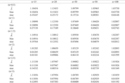
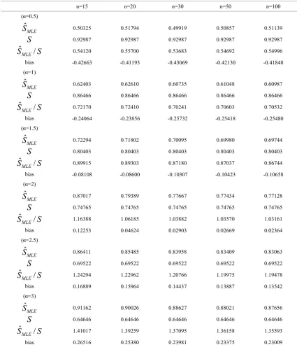
different values of α considered are 0.5, 1, 1.5, 2, 2.5 and 3. Tables (7), (8) and (9) represent the MLEs of α, λ and the s.f (

S

ˆ

_MLE) at t=0.5. We have the following comments on these tables:

 The MSE and the bias for the estimates of α and λ

decrease as the sample size increases.

 The estimation of α is better for small values of α, while the estimation of λ is better for large values of α.

 The estimated s.f increases as the value of α

increases.

 There is overestimation for both α and λ , while there

is under estimation for s.f.

3.2. Asymptotic Confidence Intervals

Here we derive the approximate CIs of the parameters that based on the asymptotic normal distribution of MLEs, since the exact distributions of the MLE of these parameters are unknown because they don’t have closed forms.

The 1st _{derivative of the log likelihood function of MGIED} is given by (3.1), (3.2), (3.3). The 2nd _{derivative is obtained} as follows

=

l( ) l nθ

∑

∑

= -= =

-+

∑

-=

n i t i n i i i

e

t

t

n

n

1 n 1 i 1

)

1

ln(

)1

(

/

ln

2

)

)

1(

1

ln(

ln

λ

α

_λ

_α

_ρ

α α ρ ρ ρ α θ

α

[1 (1 ) ]

) -(1 ] ) 1 ln( [ ) ( 2 ln 2 2 -+ -= ∂

∂ _l n n _(3.4)

∑

= -= ∂ ∂ n

i i t

t i i e t e n l

1 2 ( / )

) / (

2 ( 1 ) _{(1- )}

) ( ln 2 2 λ λ ρ ρ α λ θ

λ

(3.5)

∑

= -=

∂

∂

∂

n

i i t

t i i e t e

l

1 ( / )

) / ( ) 1 ( ) (

ln

2 λ λ

ρ

ρ

θ

λ

α

(3.6)

∑

= -= =

∂

∂

∂

n i t t i i e e n

l

1 ( / )

) / ( 2 1 ) 1 ( ] ) 1 ( 1 [ ] 1 ) 1 ln( -) -[(1 ) -(1 ) (

ln

2 λ λ α α α ρ ρ ρ α ρ ρ θ

ρ

α

_(3.7)

∑

= -= ∂ ∂ ∂ n

i i t

t i i e t e l

1 ( / ) 2

) / ( ) 1 ( ) 1 ( ) ( ln 2 λ λ ρ α θ

ρ

λ

(3.8)

The information matrix would be



















∂

∂

∂

-∂

∂

∂

-∂

∂

-=

ρ

α

θ

λ

α

θ

α

θ

θ

)

(

ln

)

(

ln

)

(

ln

)

(

2 2 2 2

l

l

l

I

ρ ρ α α λ λ ρ θ ρ λ θ ρ λ θ λ θ ρ α θ λ α θ ˆ ,ˆ ,ˆ 2 2 2 2 2 2 2 2 ) ( ln ) ( ln ) ( ln ) ( ln ) ( ln ) ( ln = = =           ∂ ∂ -∂ ∂ ∂ -∂ ∂ ∂ -∂ ∂ -∂ ∂ ∂ -∂ ∂ ∂ -l l l l l l (3.9)

The approximate (1-δ) 100% CIs for

α

,

λ

and

ρ

are: )

ˆ V( ˆ ξ _/2 α

α± δ , λˆ±ξδ_/2 V(λˆ) and ρˆ±ξδ/2 V(ρˆ) respectively, where_V(

_α

_ˆ),

_V(

_λ

_ˆ

₎

and

_V(

_ρ

_ˆ

₎

are the variances of

_α

_ˆ

,

_λ

_ˆ

and

_ρ

_ˆ

which given by the diagonal elements of _I-1₍

_θ

₎ , and

2 /

δ

ξ

is the upper (δ/2) percentile of

standard normal distribution.

4. Data Analysis

Dumonceaux and Antle (1973) used a data which represents the maximum flood level (in millions of cubic feet per second) of the Subsquenna River at Harrisburg, Pennsylvania over 20 four- year periods (1890-1969) as follows

0.645, 0.613, 0.315, 0.449, 0.297, 0.402, 0.379, 0.423, 0.379, 0.324, 0.269, 0.740, 0.418, 0.412, 0.494, 0.416, 0.338, 0.392, 0.484, 0.265

Here we want to test if this data comes from MGIED or GIED using the likelihood ratio test, which is we want to test

 H0: ρ=1 (GIED)

 H1: ρ≠1 (MGIED)

The results of this test is presented in the following table

Table 2. The estimates and the LRT statistic for the flood level data

λ

ˆ

α

ˆ

ρ

ˆ

ln l(θ) X2 p-value Under

H0 1.652 38.476 --- 15.516

109.239 1.438×10-25 Under

H1 0.278 3.818 0.0248 70.135

Note that the value of X2 _{is greater than the critical value of}

chi-square with one degree of freedom; also the very small p-value indicates that this data fits MGIED much better than GIED.

If we want to find the asymptotic CIs for the parameters of the data in this example as it comes from MGIED, we obtain the observed information matrix as





















=

9.735

70.232

-188.384

-70.232

-262.635

0.611

-188.384

-0.611

-0.001

)

(

θ

I

, and the variance covariance matrix

_I

-1

₍

_θ

₎

          × = -8 -1 10 1.036 0.000012 -0.0053 -0.000012 -0.0038 0.00142 -0.0053 -0.00142 -0.00025 ) (θ I .

The 95% CIs for α, λ, and ρ are given by [3.787, 3.849], [0.157, 0.399] and [0.0246, 0.0250] respectively.

[image:4.595.66.545.81.421.2]

The Q-Q plot of the flood level data is represented in figure 4 confirms our result, where the percentile pi is taken

to be (i-0.5/n).

5. Conclusions

[image:4.595.324.539.555.720.2]

In This paper, we introduced a new distribution that can serve better than existing well known models. The reliability and probability properties are discussed. Estimation of parameters and survival function is conducted. Finally, a real set of data is fit and is shown to be apropriate.

[image:5.595.101.515.81.730.2]

Table 3. MLEs of MGIED parameter, different levels of α(λ=1, ρ=0.8)

α 1 1.5 2 2.5 3

1.01414 0.98545 1.00612 1.03321 1.03426 0.00840 0.02997 0.02928 0.01212 0.01102 0.01414 -0.01455 0.00612 0.03321 0.03426

1.00000 2.61335 3.30387 4.19800 4.92128 1.00000 1.74223 1.65194 1.67920 1.64043 1.01*10-8 _{3.65998 7.41570 9.28547 9.40771}

1.81*10-6 _{1.11335 1.30387 1.69800 1.92128}

-- 0.20213 0.50354 0.58144 0.60140 -- 0.25266 0.62942 0.72680 0.75174 -- 0.32353 0.11294 0.09425 0.08423 -- -0.59787 -0.29646 -0.21856 -0.19861

Table 4. MLE of the reliability (survival) for MIGED (1, α,0.8), (t=1)

α 1 1.5 2 2.5 3

MLE

Sˆ _{0.63728 0.58415 0.45683 0.36138 0.29855}

S 0.63212 0.55283 0.47709 0.40776 0.34621

S

SˆMLE/ 1.00817 1.05665 0.95752 0.88626 0.86234

bias 0.00516 0.03132 -0.02026 -0.04638 -0.04766

Table 5. MLEs of MGIED parameter, different levels of ρ(λ=1, α=2)

ρ 0.2 0.4 0.6 0.8

λ

ˆ

1.01834 1.00068 1.00477 1.00612

λ

ˆ

mse

0.01999 0.02374 0.02128 0.02928

λ

ˆ

bias

0.01834 0.00068 0.00477 0.00612

α

ˆ

1.90877 2.49370 3.45538 3.30387

0

/

ˆ

α

α

0.95438 1.24685 1.72769 1.65194

α

ˆ

mse

2.94654 3.37081 5.14884 9.28547

α

ˆ

bias

-0.09123 0.49370 1.45538 1.30387

ρ

ˆ

0.09912 0.07803 0.30834 0.50354

0

/

ˆ

ρ

ρ

0.49559 0.19509 0.51389 0.62942

ρ

ˆ

mse

0.09912 0.04595 0.03604 0.11294

ρ

ˆ

bias

-0.28167 -0.32197 -0.29166 -0.29646

Table 6. MLE of the reliability (survival) for MGIED (1, 2,ρ)

ρ 0.2 0.4 0.6 0.8

MLE

S

ˆ

0.63122 0.61825 0.52941 0.45683

S 0.60628 0.57399 0.53246 0.47709

ˆ /

MLE

S S

1.04113 1.07712 0.99428 0.95752

bias 0.02493 0.04426 -0.00305 -0.02026

λ

ˆ

λˆ

mse

λˆ

bias

α

ˆ

0 / ˆ α α

αˆ mse

αˆ bias

ρˆ

0 / ˆ ρ ρ

ρ

ˆ

mse

ρ

ˆ

[image:6.595.88.517.90.442.2]

Table 7. MLE of α for MGIED whenρ is known(ρ =0.8)

n=15 n=20 n=30 n=50 n=100

(α=0.5)

αˆ 0.67641 0.66670 0.59341 0.56235 0.54624

α

α

ˆ/ 1.35283 1.33341 1.18681 1.12469 1.09248 bias 0.17641 0.16670 0.09341 0.06235 0.04624 mse 1.06566 0.83498 0.56062 0.34227 0.15966

(α=1)

α

ˆ 1.31423 1.21906 1.11259 1.07593 1.05251

α

α

ˆ/ 1.31423 1.21906 1.11259 1.07593 1.05251 bias 0.31423 0.21906 0.11259 0.07593 0.05251 mse 1.28885 0.86146 0.54612 0.29839 0.14223

(α=1.5)

α

ˆ 1.88782 1.76232 1.63981 1.59387 1.56061

α

α

ˆ/ 1.25855 1.17488 1.09321 1.06258 1.04041 bias 0.38782 0.26232 0.13981 0.09387 0.06061 mse 1.53549 0.99291 0.58809 0.31345 0.14948

(α=2)

α

ˆ 3.03601 2.32592 2.15734 2.11662 2.07228

α

αˆ/ 1.51801 1.16296 1.07867 1.05831 1.03614 bias 1.03601 0.32592 0.15734 0.11662 0.07228 mse 1.32657 1.31540 1.22991 0.37454 0.17417

(α=2.5)

αˆ 3.10827 2.91302 2.73236 2.64705 2.58813

α

α

ˆ/ 1.24331 1.16521 1.09294 1.05882 1.03525 bias 0.60827 0.41302 0.23236 0.14705 0.08813 mse 3.35949 1.89371 0.93218 0.48039 0.21663

(α=3)

αˆ 3.81486 3.54239 3.30045 3.18585 3.10840

α

α

ˆ/ 1.52594 1.41696 1.32018 1.27434 1.24336 bias 0.81486 0.54239 0.30045 0.18585 0.10840 mse 5.17168 2.68091 1.25924 0.64060 0.28007

Table 8. MLE of λ for MGIED whenρ is known (ρ =0.8)

n=15 n=20 n=30 n=50 n=100

(α=0.5)

λˆ 1.18454 1.15433 1.09799 1.05965 1.03730 bias 0.18454 0.15433 0.09799 0.05965 0.03730 mse 0.35247 0.25173 0.15716 0.08581 0.04148

(α=1)

λˆ 1.18098 1.12330 1.07449 1.04420 1.02887 bias 0.18098 0.12330 0.07449 0.04420 0.02887 mse 0.27138 0.17109 0.10648 0.05651 0.02743

(α=1.5)

λ

ˆ

1.14916 1.10012 1.05938 1.03670 1.02387 bias 0.14916 0.10012 0.05938 0.03670 0.02387 mse 0.19764 0.12552 0.07696 0.04079 0.02012

(α=2)

λ

ˆ 1.01285 1.08659 1.05129 1.03242 1.02093 bias 0.01285 0.08659 0.05129 0.03242 0.02093 mse 0.01101 0.09886 0.06110 0.03234 0.01599

(α=2.5)

λ

ˆ 1.11330 1.07947 1.04882 1.03022 1.01926 bias 0.11330 0.07947 0.04882 0.03022 0.01926 mse 0.14332 0.08514 0.05038 0.02739 0.01349

(α=3)

[image:6.595.94.516.456.736.2]

[image:7.595.91.517.91.588.2]

Table 9. MLE of the reliability (survival) for MGIED whenρ is known (ρ =0.8)(t=0.5)

n=15 n=20 n=30 n=50 n=100

(α=0.5)

MLE

S

ˆ

0.50325 0.51794 0.49919 0.50857 0.51139

S

0.92987 0.92987 0.92987 0.92987 0.92987

S

S

ˆ

MLE

/

0.54120 0.55700 0.53683 0.54692 0.54996

bias -0.42663 -0.41193 -0.43069 -0.42130 -0.41848

(α=1)

MLE

S

ˆ

0.62403 0.62610 0.60735 0.61048 0.60987

S

0.86466 0.86466 0.86466 0.86466 0.86466

S

S

ˆ

MLE

/

0.72170 0.72410 0.70241 0.70603 0.70532

bias -0.24064 -0.23856 -0.25732 -0.25418 -0.25480

(α=1.5)

MLE

S

ˆ

0.72294 0.71802 0.70095 0.69980 0.69744

S

0.80403 0.80403 0.80403 0.80403 0.80403

S

S

ˆ

MLE

/

0.89915 0.89303 0.87180 0.87037 0.86744

bias -0.08108 -0.08600 -0.10307 -0.10423 -0.10658

(α=2)

MLE

S

ˆ

0.87017 0.79389 0.77667 0.77434 0.77128

S

0.74765 0.74765 0.74765 0.74765 0.74765

S

S

ˆ

MLE

/

1.16388 1.06185 1.03882 1.03570 1.03161

bias 0.12253 0.04624 0.02903 0.02669 0.02364

(α=2.5)

MLE

S

ˆ

0.86411 0.85485 0.83958 0.83409 0.83063

S

0.69522 0.69522 0.69522 0.69522 0.69522

S

S

ˆ

MLE

/

1.24294 1.22962 1.20766 1.19975 1.19478

bias 0.16889 0.15964 0.14437 0.13887 0.13542

(α=3)

MLE

S

ˆ

0.91162 0.90026 0.88627 0.88021 0.87656

S

0.64646 0.64646 0.64646 0.64646 0.64646

S

S

ˆ

MLE

/

1.41017 1.39259 1.37095 1.36158 1.35593

bias 0.26516 0.25380 0.23981 0.23375 0.23009

REFERENCES

[1] Abouammoh A. and Alshangiti Arwa M. (2009). Reliability estimation of generalized inverted exponential distribution. Journal of Statistical Computation and Simulation, 79, 1301 - 1315

[2] Dey, Sanku (2007) Inverted exponential distribution as a life distribution model from a Bayesian viewpoint. Data Science Journal, 6, 107-113.

[3] Dumonceaux, R and Antle, C. E. (1973). Discriminating

between the lognormal and Weibull distributions. Technometrics, 15, 923-926.

[4] Hendi, M. I., Abu-yussef, S. E. and Elradadi A. (2004). Order statistic from generalized inverted exponential distribution. Egypt. Statist. Soci. , Vol 20,no.1, 57-77 [5] Gupta, R.D. and Kundu, D. (1999). Generalized

exponential distribution. Austral. N. Z. J. Statist, 41 (2),173-188

[6] Killer, A.Z. and Kamath, A. R. (1982). Reliability analysis of CNC Machine Tools, Relieb. Engng., 3, 449-473.

Gamma as Life Distribution. Microelectron. Reliab. 29, 619-626.

[8] Martinez, A. S.; González, R. S. and Terçariol, C. A. S. (2009). Generalized Probability Functions. Advances in

Mathematical Physics Volume 2009, 13 pages