AN INVENTORY MODEL FOR DETERIORATING ITEMS WITH STOCK DEPENDENT DEMAND, TIME VARYING HOLDING COST AND SHORTAGES DEPENDENT COMPLETE BACKLOGGING WITH FINITE PLANNING HORIZON

(1)

A Monthly Double-Blind Peer Reviewed Refereed Open Access International e-Journal - Included in the International Serial Directories.

GE- International Journal of Management Research (GE-IJMR)

Website: www.aarf.asia. Email: [email protected] , [email protected] Page 248

AN INVENTORY MODEL FOR DETERIORATING ITEMS WITH STOCK

DEPENDENT DEMAND, TIME VARYING HOLDING COST AND

SHORTAGES DEPENDENT COMPLETE BACKLOGGING WITH FINITE

PLANNING HORIZON

Balvinder Singh Sandhu1, Arun Kumar Tomer2

1

Lovely Professional University, Phagwara, Punjab-India.

2

SMDRSD College, Pathankot. Punjab-India.

ABSTRACT

This paper presents inventory model for perishable items with inventory level dependent demand rate. It is assumed that shortages are allowed and completely backlogged. It is assumed that the deterioration of the item does not begin at the instant of the arrivals in stock. It begins after some fixed time. Profit function has been established and objective is to maximize the total average profit per unit time. Finite planning horizon is considered. The results are illustrated with the help of numerical examples. The sensitivity of the solution with the change of the values of the parameters associated with the model is also discussed.

Keywords: Inventory, Stock-dependent demand, shortages, deterioration, backlogging, finite

planning horizon

___________________________________________________________________________

1. Introduction

(2)

GE- International Journal of Management Research (GE-IJMR)

that product. Displayed stock level plays an important role to attract customers. For certain types of goods, particularly for consumer goods, the demand is proportional to the stock level. If the demand rate is dependent on the stock level, there may two factors need to consider when establishing models. One is, when a product is highly perishable, the seller may prefer to backlog demand in order. But not all customers are ‘‘patient’’, some customers may accept backlogging

during the shortage period, while the others would not. Hence only a fraction of demand occurring at a given time is backordered. The fraction, moreover, is a decreasing function of the amount of demand already backlogged and the waiting time. The more the amount of demand backlogged, the smaller the demand to accept backlogging would be. Meanwhile, the willingness of a customer to wait for backlogging during a shortage period is declined with the length of the waiting time. Secondly, if the demand is dependent on the inventory level, an increase in shelf space for an item can induce more consumers to buy it. This occurs because of its visibility, popularity or variety. Conversely, low stocks of certain goods. (e.g., food) might raise the perception that they are not fresh. Therefore, building up inventory often has a positive impact on the sales, as well as the profit.

Due to the facts, a number of researchers have developed the EOQ models that focused on stock- dependent demand rate pattern. Recently, Zhou, Min, and Goyal [1] studied the coordination of supply chain with power-form inventory-level-dependent demand. Padmanabhan and Vrat[2] presented an inventory model for deteriorating items with stock dependent selling rate and derived the profit functions without backlogging, with partial backlogging and with complete backlogging. Alfares [3] proposed the inventory model with stock-level dependent demand rate and variable holding cost. Hou [4] developed an inflation model for deteriorating items with stock-dependent consumption rate and completely backordered shortages by assuming a constant length of replenishment cycles and a constant fraction of the shortage length with respect to the cycle length. Recently, Wu and Zhao [16] discussed supplier retailer inventory coordination with credit term for inventory-dependent and linear-trend demand.

(3)

GE- International Journal of Management Research (GE-IJMR)

Photographic goods, Electronic goods, Chemical based stocks deteriorate through a gradual loss of utility with the passage of time, so deterioration of physical goods in stock as a very realistic feature and it is necessary to incorporate this factor into research.

Recently, Hou and Lin [5] and Jolai, Tavakkoli-Moghaddam, Rabbani, and Sadoughian [6] incorporated effects of deterioration and stock-dependent demand rates to develop a finite time horizon inventory/production model under inflation. Soni and Shah [7] proposed a deterministic inventory model with stock-dependent demand under trade credit policy. In most of the inventory models, holding cost is known and is considered as constant. But in real life situation holding cost need not be a constant as because other parameters may govern the holding cost. In generalization of EOQ models, various functions describing holding cost were considered by several researchers like Giri, Goswami and Chaudhuri [8] Naddor [9], Weiss [10] and Goh [11],Van Der Veen [12],. Muhlemann and Valtis-Spanopoulos [13] treated the holding cost as a non-linear function of the length of the time for which the item is held in stock and as a functional form of the amount of the on-hand inventory. Roy [14] developed an EOQ model for deteriorating items where deterioration rate and holding cost are expressed as linearly increasing functions of time and demand rate is a function of selling price and shortages are allowed and completely backlogged. Sahoo et al. [15] also considered time varying holding cost with constant deterioration.

In this paper we analyze a deterministic inventory model assuming that demand is stock-dependent during the finite planning horizon. In addition holding cost is assumed to be time varying, shortage are fully backlogged and the products have a deterioration process after a certain period of time. The organization of the paper is as follows: In section 2, we introduce the notation used throughout the paper and the basic assumptions of the inventory system, in section 3, we develop the mathematical model that describes the evolution of the inventory system and a procedure to solve the inventory problem is presented, in section 4, numerical example is provided to illustrate the solution procedure, in section 5, we present a sensitivity analysis of the inventory policy and in last the conclusion is discussed.

(4)

GE- International Journal of Management Research (GE-IJMR)

The following notations are used throughout the paper.

2.1. Notations:

) (t

I : the inventory level at time t.

D(I) : the demand rate which is a function of the on hand inventory level I(t). (CH )(t) : holding cost at time t.

 : constant rate of deterioration.

CU : purchasing cost i.e. the cost of the inventory item/ unit.

CS : shortage cost, cost/unit/unit time.

CR : the replenishment cost/ replenishment.

t1 : time when deterioration starts.

t2 : time when inventory level falls to zero due to demand and deterioration.

Ti : length of the i

th

replenishment cycle.

max

I : the maximum inventory level for each ordering cycle.



I : the inventory level when deterioration starts.

d

I : total amount of deteriorated items.

Q : the order quantity for each ordering cycle.

Q

B : total amount of backorder.

P : the selling price of item/unit item.

H : the planning horizon

2.2. Assumptions:

1. The inventory system involves only one item. 2. Planning horizon is finite.

3. The replenishment rate is infinite and instantaneous but replenishment size is finite. 4. The deterioration rate (0 1)is constant.

(5)

6. The demand rate

  

  



0 ) ( ,

0 ) ( , ) ( )

(

t I a

t I t

bI a I D

i i

, where a>0 is initial demand and

0<b<1is a constant.

7. Holding cost per item per unit time is time dependent and is assumed to be as

0 , 0 ; , )

(t t where    C_H

8. The deterioration function is assumed to be (t).i(tt1)where (0< <<1)is

constant and _i(tt₁)is defined as

  

 

  



 

1 1

1 1 1

, 0

, 1 ) (

t T t

t T t t

t

i i i

 , where t is the time

measured from the instant of arrival of a fresh replenishment indicating that the deterioration of the items begins after a time from the instant of that arrival in stock

9. Shortages are allowed and completely backlogged.

3. Model formulation and development

let I(t) the inventory level at any time t. The inventory is depleted partly to meet the demand and partly for deterioration during the period of positive inventory. The behavior of inventory system during the finite planning horizon at any time is depicted in figure:

inventory

.

Imax Imax Imax I(t) Imax Imax

I_ …… I I …… I

t=t0 t=t1 t=t2 t=H/m t=(i-1)H/m t=(i)H/m t=(i+1)H/m t=H time

Ti-1 Ti Ti+1

(6)

GE- International Journal of Management Research (GE-IJMR)

Figure shows basic information about the inventory during the planning horizon. First replenishment is made at a time t=0 and inventory level is at its maximum Imax. The inventory

level decreases gradually due to demand. After time t1, inventory level decreases gradually due to

both demand and deterioration and ultimately falls to zero at t = t2 . Let m+1 be the number of

replenishments to be made during planning horizon H. To clear up the backlog, the last replenishment is made at time t=H. The length of each replenishment is H/m. The ith cycle starts

at time

m M i

t( 1) =Ti-1 and ends at time

m M i

t( ) = Ti .Thereafter deterioration starts at time

1 1 t

T

t i and shortages start at time tTi1t2 (i=1,2,3…….m) .The rate of change of inventory

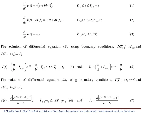
level during the ith cycle positive stock period [T_i_₁,T_i_₁t₁] then [T_i_₁t₁,T_i_₁t₂] and during negative stock period [T_i_₁t₂,T_i] i.e. shortage period, can be described by the following differential equations:



( )



)

(t a bI t I

dt d

 

 , T_i_₁tT_i_₁t₁ (1)



( )



) ( )

(t I t a bI t I

dt d

  

 , T_i_₁t₁ tT_i_₁t₂ (2)

a t I dt

d __ )

( , T_i_₁t₂tT_i (3)

The solution of differential equation (1), using boundary conditions, I(T_i_₁)I_maxand



I t T

I( i1 1)

b a e I b a t

I  bt

  

  

 

max

)

( , T_i_₁tT_i_₁t₁ (4) and

b a e I b a

I  bt 

  

  

  1

max

 (5)

The solution of differential equation (2), using boundary conditions, I(T_i_₁t₂)0and



I t T

I( i1 1)

  





b e a t I

t t b

 

  



1 )

(

2

, Ti1t1tTi1t2 (6) and

  





b e

a I

t t b

 

  



 1

1 2

[image:6.612.70.544.343.720.2]

(7)

GE- International Journal of Management Research (GE-IJMR)

From equations (5) and (7) we get,

  









b e a b e e a I bt bt t t b 1

1 1 1

1 2 max          (8)

The net profit for the ith cycle is

) , ( ) ( )

(PF i  PF i t2 m = (Net inventory after excluding deteriorated inventory) x selling unit price

+ (selling price of item - the cost of the inventory item ) x total amount of backorder at the end of cycle - Purchasing cost - Holding cost-Shortage cost - Replenishment cost)

Calculation of variable costs:

Holding cost



      2 1 1 2 ) ( ) ( ) ( ) ( ) ( ) ( ) ( 0 0 t t t t i

H t I t dt t I t dt t I t dt

C      















  



  

















b b t T a b t a b b t a b b T e a b t a b t b T a b b t a e b e b b T a b b T e a i i bt i t t b t t b i i bt ) ( ) ( ) ( 2 ) ( ) ( 1 ) ( 2 ) ( ) )( ( ) ( ) ( 1 ) ( ) )( ( ) ( 1 1 1 2 1 1 2 1 2 2 2 2 1 2 1 2 1 2 1 1 1 2 1 2 1                                                                             

For simplification, take

b

s  ,







₂ 1



(8)

Therefore,









_i _i

t t s t

t s i i

i

H t t

s e s

e

C ) ( ) ( ) 1 ( ) ( )

( ₂ ₂ ₄ ₂2 ₅

) ( 3 )

( 2 1

1 2 1

2

      

  

 

  

Shortage cost





T

t S

Sh C I t dt

C

2

)

( /2

2

2

  



 _



 t

m H a C_s

Amount of deteriorated inventory







 

 2

1

) (

t

d I a bI t dt

I _

  











b



t t a b

e a b t t

  

 

  

  

 

1 2 2

1

1 2

Total amount of backorder at the end of thecycle is

   



 _

 t2

m H a BQ

)

( ₂

max a T t

I

Q  



Therefore the net profit for the ith cycle is



d U Q U H i Sh R



i

i PF t m I I P P C B I C C C C

PF) ( )( , ) (  ) (  )  . ( )  

( ₂ _max _max (*)

(9)

GE- International Journal of Management Research (GE-IJMR)

                                         _ _ _           _         _          _ _        _ _ _    _   R U bt i i i U bt bt U S i t t s i i U bt bt i C s t aP b C P e a s s C ae s P a s P ae t m H C P a t m H a C t t s P a e s s s C ae s P a s P ae PF 1 5 2 1 2 2 2 2 2 2 4 2 2 3 2 1 2 ) )( 1 ( ) ( ) ( ) ( ) ( 2 ) ( ) ( ) ( ) ( 1 1 1 1 2 1 1    

For Simplification, take

s s C ae s P a s P

ae U i i

bt bt i ) ( ) ( )

( 1 2

2 6

1

1   

      , s 3 7    , s P a i i      ) ( )

( 8 2

R U bt i i i U bt bt i C s t aP b C P e a s s C ae s P a s P

ae _ _ _   _ _

      _ _ _       1 5 2 1 2 9 ) )( 1 ( ) ( ) ( ) ( ) ( 1 1

1  

Therefore (PF)i becomes





                      _         _           i U S i t t s i i t m H C P a t m H a C t t e

PF ( ) ( )

2 ) ( ) ( )

( 2 9

2 2 2 2 4 2 8 7

6 2 1 (9)

Now, net profit for the entire period ‘H’ is



     m i i R PF t m

C m t TPF TPF 1 2

2, ) ( ) ( , )

)( (  









    _ _                     _         _          m i i U S m i i m i i t t s m t m H C P a t m H a C t t e 1 9 2 2 2 2 2 4 1 8 2 1 7

6 ( ) ( )

(10)

GE- International Journal of Management Research (GE-IJMR)

 





m C P a t m H a C t se TPF dt d U S m i i m i i t t s       _ _       _         



   ) ( 2 ) ( )

( ₄₂ ₂

1 8 1 7 6 2 1 2  



 



m a C e s TPF dt d S m i i t t

s _ __ _ _ _





  4 1 7 6 2 2 2 2 2 ) ( 1 2

Now for maximum TPF, we must have 0

2

 TPF dt

d

and satisfying ₂ 0

2 2  TPF dt d (11) Now, 0 2  TPF dt d gives  





0 ) ( 2 ) ( )

( 4 2 2

1 8 1 7 6 1 2        _ _       _        



   m C P a t m H a C t

se S U

m i i m i i t t s (12)

Equations (12) is a nonlinear equations in t2, this can be solved for t2 and obtained value of t2

must satisfy condition (11) to maximize the total profit per time unit.After satisfying the

condition (11) the optimal solutions are obtained.

4. Numerical example

Suppose that there is a product with stock dependent demand and other parameters of the inventory system are a=30,b=0.1, 0.03,t1=0.5,CU=7,CS=

0.4, CR=30, =0.4, =0.02, P=10,

H=20 days. Using these values of parameters we get different values of t2 and TPF for different values of

m=1,2,3,…….From the table optimal

value of m=m*=7, t₂ t₂*=1.2721 and TPF=TPF* =1377.69 .

m t2 TPF

1 7.7514 392.66

2 4.1067 1040.74

3 2.8185 1238.69

4 2.1530 1322.33

5 1.7457 1360.30

6 1.4705 1375.49

7 1.2721 1377.69

8 1.2228 1371.78

9 1.0051 1360.48

(11)

After obtaining these values, we get the optimal maximum level I*max = 41.271and the optimal

order quantity Q* = 88.821.

5. Sensitivity Analysis

(12)

Website: www.aarf.asia. Email: [email protected] , [email protected] Page 259 Parameter %change

a t2* Imax* Q* TPF* t2* Imax* Q* TPF*

15 50% 1.2721 61.9065 133.2320 2186.5300 0.0000 50.0000 50.0002 58.7099

37.5 25% 1.2721 51.5888 111.0270 1782.1100 0.0000 25.0001 25.0006 29.3549

30 0% 1.2721 41.2710 88.8212 1377.6900 0.0000 0.0000 0.0000 0.0000

22.5 -25% 1.2721 30.9533 66.6159 973.2650 0.0000 -24.9999 -25.0000 -29.3553

15 -50% 1.2721 20.6355 44.4106 568.8430 0.0000 -50.0000 -50.0000 -58.7104

b

0.15 50% 1.5019 51.4424 92.1010 1408.3300 18.0587 24.6454 3.6926 2.2240

0.125 25% 1.3761 45.7583 90.1902 1391.5500 16.1837 21.6080 2.7107 1.8704

0.1 0% 1.2721 41.2710 88.8212 1377.6900 0.0000 0.0000 0.0000 0.0000

0.075 -25% 1.1844 37.6277 87.8099 1366.0000 -6.8963 -8.8277 -1.1386 -0.8485

0.05 -50% 1.1091 34.6044 87.0450 1355.9900 -12.8139 -16.1532 -1.9997 -1.5751

θ

0.045 50% 1.1578 37.5079 88.4883 1365.4100 -8.9873 -9.1180 -0.3748 -0.8913

0.0375 25% 1.2118 39.2843 88.6453 1371.2000 -4.7448 -4.8138 -0.1980 -0.4711

0.03 0% 1.2721 41.2710 88.8212 1377.6900 0.0000 0.0000 0.0000 0.0000

0.0225 -25% 1.3401 43.5073 89.0196 1384.9800 5.3399 5.4186 0.2234 0.5291

0.015 -50% 1.4171 46.0425 89.2450 1393.2600 11.3927 11.5614 0.4771 1.1302

CU

10.5 50% 0.8662 27.3598 87.0875 -772.8490 -31.9078 -33.7070 -1.9519 -156.0975

8.75 25% 1.0283 32.8281 87.6921 297.3330 -19.1639 -20.4572 -1.2712 -78.4180

7 0% 1.2721 41.2710 88.8212 1377.6900 0.0000 0.0000 0.0000 0.0000

5.25 -25% 1.6833 56.1297 91.3459 2478.8800 32.3190 36.0028 2.8425 79.9302

3.5 -50% 2.5478 90.0895 99.3697 3635.8800 51.3602 60.5024 8.7840 46.6743

CS

0.6 50% 1.5358 50.7094 90.3489 1333.7400 20.7282 22.8693 1.7200 -3.1901

0.5 25% 1.4167 46.4058 89.6187 1353.7200 11.3652 12.4417 0.8979 -1.7399

0.4 0% 1.2721 41.2710 88.8212 1377.6900 0.0000 0.0000 0.0000 0.0000

0.3 -25% 1.0922 35.0123 87.9618 1407.0500 -14.1471 -15.1649 -0.9676 2.1311

0.2 -50% 0.8603 27.1626 87.0676 1444.0400 -32.3725 -34.1848 -1.9743 4.8160

CR

45 50% 1.2721 41.2710 88.8212 1257.6900 0.0000 0.0000 0.0000 -8.7102

37.5 25% 1.2721 41.2710 88.8212 1317.6900 0.0000 0.0000 0.0000 -4.3551

30 0% 1.2721 41.2710 88.8212 1377.6900 0.0000 0.0000 0.0000 0.0000

22.5 -25% 1.2721 41.2710 88.8212 1437.6900 0.0000 0.0000 0.0000 4.3551

15 -50% 1.2721 41.2710 88.8212 1497.6900 0.0000 0.0000 0.0000 8.7102

α

0.6 50% 1.0438 33.3539 87.7556 1348.3800 -17.9526 -19.1832 -1.1997 -2.1275

0.5 25% 1.1465 36.8855 88.2058 1361.5500 -9.8779 -10.6261 -0.6929 -1.1715

0.4 0% 1.2721 41.2710 88.8212 1377.6900 0.0000 0.0000 0.0000 0.0000

0.3 -25% 1.4297 46.8703 89.6949 1397.9300 12.3832 13.5672 0.9837 1.4691

0.2 -50% 1.6334 54.2851 90.9971 1424.1400 28.3996 31.5333 2.4498 3.3716

β

0.03 50% 1.1563 37.2270 88.2515 1363.0900 -9.1028 -9.7986 -0.6414 -1.0597

0.025 25% 1.2113 39.1372 88.5141 1370.0200 -4.7857 -5.1702 -0.3458 -0.5567

0.02 0% 1.2721 41.2710 88.8212 1377.6900 0.0000 0.0000 0.0000 0.0000

0.015 -25% 1.3401 43.6732 89.1842 1386.2100 5.3438 5.8206 0.4087 0.6184

0.01 -50% 1.4166 46.4021 89.6181 1395.7600 11.3573 12.4327 0.8972 1.3116

P

15 50% 2.9293 106.3330 104.1680 4589.5200 106.7824 129.1556 16.2354 228.8187

12.5 25% 1.7598 58.9832 91.9043 2940.3900 38.3326 42.9168 3.4711 113.4290

10 0% 1.2721 41.2710 88.8212 1377.6900 0.0000 0.0000 0.0000 0.0000

7.5 -25% 0.9991 31.8332 87.5745 -157.3350 -21.4624 -22.8679 -1.4036 -111.4202

5 -50% 0.8235 25.9386 86.9473 -1679.7800 -35.2646 -37.1505 -2.1097 -221.9273

(13)

GE- International Journal of Management Research (GE-IJMR)

On the basis of the results shown in above table, the following observations can be made.

1. With the increase in the value of parameter a, Imax*, Q* and TPF* increase and

these parameters are very sensitive to change in parameter a .

2. With the increase in the value of parameter b, t2* , Imax*,Q* and TPF* increase and

Imax* and Q* are sensitive to change in b.

3. With the increase in the value of parameter θ, t2* , Imax*,Q* and TPF* decrease and

Imax* and TPF* are sensitive to change in parameter θ.

4. t2* , Imax*,Q* and TPF* decrease with the change in the value of parameter CU. Imax*

is sensitive to change in CU whereas TPF* is very sensitive to change in CU.

Moreover when we increase the unit cost by 50% while other parameters remains constant, the system will go in loss.

5. With the increase in the value of parameter CS, t2* , Imax* and Q* increase while

TPF* decrease . t2*, Imax* and TPF* are sensitive to change in CS. while Q* is low

sensitive to change in CS.

6. TPF* decreases with the change in the value of parameter CR. TPF* is also

sensitive to change in CR while t2* , Imax*,Q* has almost no change with the change

in CR.

7. With the increase in the value of parameter α, t2* , Imax*,Q* and TPF* decrease and

Imax* and TPF* are sensitive to change in parameter α.

8. t2* , Imax*,Q* and TPF* decrease with the change in the value of parameter β. and

are low sensitive to change in β

9. t2* , Imax*,Q* and TPF* increase with the increase in the value of parameter P. and

(14)

GE- International Journal of Management Research (GE-IJMR)

6. Conclusion and Future research

In this proposed model, we present a deterministic inventory model with stock dependent demand and time varying holding cost, allowing shortages with complete backlogging is considered. Deterioration of items starts after some time and rate of deterioration is constant. This type of model is useful for all such items where deterioration of items begin after a specific time from the instant of their arrival in stock. Different results of calculus have been used to establish the model.

The present model may be extended in several ways. For instance, we may extend the model to allow for a varying rate of deterioration. Additionally, we could consider Price dependent demand, stock dependent holding cost.

Acknowledgement

Numerical calculations have been done with the help of mathematical softwares Wolfram Mathematica 8.0, MATLAB 7.0 and special thanks to my fellow colleagues who helped me in using this software.

7. References

[1] Zhou, Y. W., Min, J., & Goyal, S. K. (2008). Supply-chain coordination under an inventory-level-dependent demand rate. International Journal of Production Economics, 113, 518–527.

[2] G. Padmanabhan, Prem Vrat, EOQ models for perishable items under stock dependent selling rate, European J. Oper. Res. 86 (1995) 281–292.

[3] Alfares, H.K., 2007. Inventory model with stock-level dependent demand rate and variable holding cost. International Journal of Production Economics 108 (1–2), 259– 265.

(15)

GE- International Journal of Management Research (GE-IJMR)

[5] Hou, K. L., & Lin, L. C. (2006). An EOQ model for deteriorating items with price- and stock-dependent selling rates under inflation and time value of money. International Journal of Systems Science, 37, 1131–1139.

[6] Jolai, F., Tavakkoli-Moghaddam, R., Rabbani, M., & Sadoughian, M. (2006). Aneconomic production lot size model with deteriorating items, stock-dependent demand, inflation, and partial backlogging. Applied Mathematics andComputation, 181, 380–389.

[7] Soni, H., & Shah, N. H. (2008). Optimal ordering policy for stock-dependent demand under progressive payment scheme. European Journal of Operational Research,184, 91– 100.

[8] Giri, B.C., Pal, S., Goswami, A., Chaudhuri, K.S.: An inventory model for deteriorating items with stock-dependent demand rate. Eur. J. Oper. Res. 95(3), 604–610 (1996) [9] Naddor, E.: Inventory Systems. Wiley, New York (1966)

[10] Weiss, H.J.: Economic order quantity models with nonlinear holding cost. Eur. J. Oper. Res. 9(1), 56–60 (1982)

[11] Goh, M.: EOQ models with general demand and holding cost functions. Eur. J. Oper. Res. 73(1), 50–54(1994)

[12] Van Der Veen, B.: Introduction to the Theory of Operational Research. Philip Technical Library.Springer, New York (1967)

[13] Muhlemann, A.P., Valtis-Spanopoulos, N.P.: A variable holding cost rate EOQ model. Eur. J. Oper.Res. 4(2), 132–135 (1980)

[14] Roy, A.: An inventory model for deteriorating items with price dependent demand and time-varying holding cost. Adv. Model. Optim. 10(1), 25–37 (2008)

[15] Sahoo, N.K., Sahoo, C.K., Sahoo, S.K.: An inventory model for constant deteriorating items with price dependent demand and time varying holding cost. Int. J. Comput. Sci. Commun. 1(1), 267–271 (2010)

[16] Wu Chengfeng, Zhao Qiuhong: Supplier-retailer inventory coordination with credit term for inventory-dependent and linear- trend demand.Int. Trans.in Op. Res.,797-818(2014)

25%1.7598