R E S E A R C H
Open Access
General viscosity iterative approximation
for solving unconstrained convex
optimization problems
Peichao Duan
*and Miaomiao Song
*Correspondence:
[email protected] College of Science, Civil Aviation University of China, Tianjin, 300300, China
Abstract
In this paper, we combine a sequence of contractive mappings{hn}with the proximal operator and propose a generalized viscosity approximation method for solving the unconstrained convex optimization problems in a real Hilbert spaceH. We show that, under reasonable parameter conditions, our algorithm strongly converges to the unique solution of a variational inequality problem. Our result presented in the paper improves and extends the corresponding results reported by many authors recently.
MSC: 47H09; 47H10; 47J20; 47J25; 49M05; 65J20
Keywords: contractive mapping; nonexpansive mapping; proximal operator; variational inequality problem
1 Introduction
Since the inception in , the unconstrained minimization problem (.) has received much attention due to its applications in signal processing, image reconstruction and in particular in compressed sensing. In this paper, letH be a Hilbert space with the inner product,and the induced norm · . Let(H) be the space of convex functions inH that are proper, lower semicontinuous and convex. We will deal with the convex uncon-strained optimization problem of the following type:
min
x∈Hf(x) +g(x), (.)
wheref,g∈(H). In general,f is differentiable andgis subdifferential.
As we know, problem (.) was first studied in [] and provided a nature vehicle to study various generic optimization models under a common framework. Many methods have been already proposed to solve problem (.) (see [–]). Many important classes of op-timization problems can be cast in this form, and problem (.) is a common problem in control theory. See, for instance, [] as a special case of (.) where due to the involvement of thelnorm which promotes sparsity that we can get a good result on solving the cor-responding problem. We mention in particular the classical works developed by [] and [], where a lot of weak convergence results have been discussed.
Definition .(see [, ]) The proximal operator ofϕ∈(H) is defined by
proxϕ(x) =arg min
ν∈H
ϕ(ν) +
ν–x
, x∈H.
The proximal operator ofϕof orderλ> is defined as the proximal operator ofλϕ, that is,
proxλϕ(x) =arg min
ν∈H
ϕ(ν) +
λν–x
, x∈H.
Lemma .(see []) Let f,g∈(H).Let x∗∈H andλ> .Assume that f is finite-valued and differential on H.Then x∗ is a solution to(.)if and only if x∗solves the fixed point equation
x∗=proxλg(I–λ∇f)x∗. (.)
The fixed point equation (.) immediately yields the following fixed point algorithm which is also known as the proximal algorithm [] for solving (.) as follows.
Initializex∈Hand iterate
xn+=
proxλng(I–λn∇f)
xn, (.)
where{λn}is a sequence of positive real numbers. Meanwhile, in [], the authors
Com-bettes and Wajs also proved that the algorithm converged weakly. Recently, Xu [] intro-duced the relaxed proximal algorithm.
Initializex∈Hand iterate
xn+= ( –αn)xn+αn
proxλng(I–λn∇f)
xn, (.)
where{αn}is the sequence of relaxation parameters and{λn}is a sequence of positive real
numbers, and obtain weak convergence.
However, it is well known that strongly convergent algorithms are very important for solving infinite dimensional problems and viscosity can effectively transfer weak conver-gence of certain iterative algorithm to converconver-gence strongly under appropriate conditions. Recently, based on an idea introduced in the work of Moudafi and Thakur [], Yaoet al. [], Shehu [] and Shehuet al.[, ] proposed some iteration algorithms for solving proximal split feasibility problems which are related to problem (.). They obtained strong convergence.
In this paper, motivated by works [, –], we combine a consequence of contractive mappings{hn}with the proximal operator and propose a generalized viscosity
2 Preliminaries
We adopt the following notations. LetT:H→Hbe a self-mapping ofH.
() xn→xstands for the strong convergence of{xn}tox;xnxstands for the weak
convergence of{xn}tox.
() UseFix(T)to denote the set of fixed points ofT; that is,Fix(T) ={x∈H:Tx=x}. () ωw(xn) :={x:∃xnjx}denotes the weakω-limit set of{xn}.
In this paper, in order to prove our result, we collect some facts and tools in a Hilbert spaceH. We shall make full use of the following lemmas, definitions and propositions in a real Hilbert spaceH.
Lemma . Let H be a real Hilbert space.There holds the following inequality:
x–y≤ x+ x+y,y, ∀x,y∈H.
Recall that given a closed subsetCof a real Hilbert spaceH, for anyx∈H, there exists a unique nearest point inC, denoted byPCx, such that
x–PCx ≤ x–y for ally∈C.
SuchPCxis called the metric (or the nearest point) projection ofHontoC.
Lemma .(see []) Let C be a nonempty closed convex subject of a real Hilbert space H. Given x∈H and z∈C,then y=PCx if and only if we have the relation
x–y,y–z ≥ for all z∈C.
Definition . A mappingF:H→His said to be:
(i) Lipschitzian if there exists a positive constantLsuch that
Fx–Fy ≤Lx–y, ∀x,y∈H.
In particular, ifL= , we sayFis nonexpansive, namely
Fx–Fy ≤ x–y, ∀x,y∈H;
ifL∈(, ), we sayFis contractive, namely
Fx–Fy ≤Lx–y, ∀x,y∈H.
(ii) α-averagedmapping (α-avfor short) if
F= ( –α)I+αT,
whereα∈(, )andT:H→His nonexpansive.
(i) I–his( –ρ)-strongly monotone:
(I–h)x– (I–h)y,x–y≥( –ρ)x–y, ∀x,y∈H.
(ii) I–Tis monotone:
(I–T)x– (I–T)y,x–y≥, ∀x,y∈H.
Lemma .(see [], Demiclosedness principle) Let H be a real Hilbert space,and let T:H→H be a nonexpansive mapping withFix(T)= ∅.If{xn}is a sequence in H weakly
converging to x and if{(I–T)xn}converges strongly to y,then(I–T)x=y;in particular,if
y= ,then x∈Fix(T).
Lemma .(see [] or []) Assume that{sn}is a sequence of nonnegative real numbers
such that
sn+≤( –γn)sn+γnδn, n≥,
sn+≤sn–ηn+ϕn, n≥,
where{γn}is a sequence in(, ), (ηn)is a sequence of nonnegative real numbers and(δn)
and(ϕn)are two sequences inRsuch that
(i) ∞n=γn=∞;
(ii) limn→∞ϕn= ;
(iii) limk→∞ηnk= implieslim supk→∞δnk≤for any subsequence(nk)⊂(n).
Thenlimn→∞sn= .
Proposition . (see []) If T,T, . . . ,Tn are averaged mappings, we can get that
TnTn–· · ·Tis averaged.In particular,if Tiisαi-av,i= , ,whereαi∈(, ),then TTis (α+α–αα)-av.
Proposition .(see[]) If f :H→Ris a differentiable functional,then we denote by
∇f the gradient of f.Assume that∇f is Lipschitz continuous on H. The operator Vλ=
proxλg(I–λ∇f)is+λL-av for each <λ<L.
Lemma . The proximal identity
proxλϕx=proxμϕ μ
λx+ – μ λ
proxλϕx
(.)
holds forϕ∈(H),λ> andμ> .
3 Main results
In this section, we combine a sequence of contractive mappings and apply a more gener-alized viscosity iterative method for approximating the unique fixed point of the following variational inequality problem:
(I–h)x∗,x˜–x∗≥, ∀˜x∈Fix(Vλ), (.)
Suppose that the contractive sequence{hn(x)}is uniformly convergent for anyx∈D,
whereDis any bounded subset ofH. The uniform convergence of{hn(x)}onDis denoted
byhn(x)⇒h(x) (n→ ∞),x∈D.
Theorem . Let f,g∈(H)and assume that(.)is consistent.Let{hn(xn)} be a
se-quence ofρn-contractive self-maps of H with≤ρl=lim infn→∞ρn≤lim supn→∞ρn= ρu< and Vλn=proxλng(I–λn∇f),where∇f is L-Lipschitzian.Assume that{hn(x)}is
uni-formly convergent for any x∈D,where D is any bounded subset of H.Given x∈H and define the sequence{xn}by the following iterative algorithm:
xn+=αnhn(xn) + ( –αn)Vλnxn, (.)
whereλn∈(,L),αn∈(,+λnL).Suppose that
(i) limn→∞αn= ;
(ii) ∞n=αn=∞;
(iii) <lim infn→∞λn≤lim supn→∞λn<L.
Then{xn}converges strongly to x∗,where x∗is a solution of(.),which is also the unique
solution of the variational inequality problem(.).
Proof LetSbe a nonempty solution set of (.). Step. Show that{xn}is bounded.
For anyx∗∈S,
xn+–x∗
=αnhn(xn) + ( –αn)Vλnxn–x
∗
=αn
hn(xn) –x∗
+ ( –αn)
Vλnxn–x∗
≤αnhn(xn) –hn
x∗+αnhn
x∗–x∗
+ ( –αn)Vλnxn–x∗
≤αnρnxn–x∗+αnhn
x∗–x∗+ ( –αn)xn–x∗
≤αnρuxn–x∗+αnhn
x∗–x∗+ ( –αn)xn–x∗
= –αn( –ρu)xn–x∗+αn( –ρu)
hn(x∗) –x∗
–ρu
. (.)
From the uniform convergence of{hn}onD, it is easy to get the boundedness of{hn(x∗)}.
Thus there exists a positive constantM such thathn(x∗) –x∗ ≤M. By induction, we obtain
xn–x∗≤max
x–x∗, M –ρu
,
which implies that the sequence{xn}is bounded.
Step. Show that for any sequence (nk)⊂(n),
lim
Firstly, note that from (.) we have
xn+–x∗
=αnhn(xn) + ( –αn)Vλnxn–x∗
=αn
hn(xn) –x∗
+ ( –αn)
Vλnxn–x∗
=αnhn(xn) –x∗
+ ( –αn)Vλnxn–x∗
+ αn( –αn)
hn(xn) –x∗,Vλnxn–x∗
≤αnhn(xn) –hn
x∗+hn
x∗–x∗
+ ( –αn)Vλnxn–x∗+ αn( –αn)
hn(xn) –x∗,Vλnxn–x∗
≤αnρnxn–x∗+hn
x∗–x∗
+ ( –αn)Vλnxn–x
∗+ α
n( –αn)
hn(xn) –x∗,Vλnxn–x
∗
≤αnρnxn–x∗
+hn
x∗–x∗+ αn( –αn)ρnxn–x∗
+ ( –αn)Vλnxn–x
∗+ α
n( –αn)
hn
x∗–x∗,Vλnxn–x
∗
= –αn
–αn
+ ρn
– ( –αn)ρnxn–x∗
+ αnhn
x∗–x∗+ αn( –αn)
hn
x∗–x∗,Vλnxn–x∗
. (.)
Secondly, sinceVλnis
+λnL
-av, we can rewrite
Vλn=proxλng(I–λn∇f) = ( –wn)I+wnTn, (.)
wherewn=+λnL,Tnis nonexpansive and, by condition (iii), we get <lim infn→∞wn≤
lim supn→∞wn< . Thus, we have from (.) and (.)
xn+–x∗
=αnhn(xn) + ( –αn)Vλnxn–x
∗
=Vλnxn–x
∗+α
n
hn(xn) –Vλnxn
=Vλnxn–x∗
+αnhn(xn) –Vλnxn
+ αn
Vλnxn–x∗,hn(xn) –Vλnxn
=( –wn)xn+wnTnxn–x∗
+αnhn(xn) –Vλnxn
+ αn
Vλnxn–x∗,hn(xn) –Vλnxn
= ( –wn)xn–x∗+wnTnxn–Tnx∗–wn( –wn)Tnxn–xn
+αnhn(xn) –Vλnxn
+ αn
Vλnxn–x∗,hn(xn) –Vλnxn
≤xn–x∗–wn( –wn)Tnxn–xn+αnhn(xn) –Vλnxn
+ αn
Vλnxn–x
∗,h
n(xn) –Vλnxn
. (.)
Set
sn=xn–x∗
, γn=αn
–αn
+ ρn
– ( –αn)ρn
,
δn=
–αn( + ρn) – ( –αn)ρn
αnhn
+ ( –αn)
hn
x∗–x∗,Vλnxn–x
∗,
ηn=wn( –wn)Tnxn–xn,
ϕn=αnhn(xn) –Vλnxn
+ αn
Vλnxn–x
∗,h
n(xn) –Vλnxn
,
sinceγn→,
∞
n=γn=∞(limn→∞( –αn( + ρn) – ( –αn)ρn) = ( –ρu) > ) and ϕn→ (αn→) hold obviously, so in order to complete the proof by using Lemma .,
it suffices to verify thatηnk→ (k→ ∞) implies that
lim sup
k→∞
δnk≤
for any subsequence (nk)⊂(n).
Indeed, ηnk → (k→ ∞) implies thatTnkxnk –xnk → (k→ ∞) due to
condi-tion (iii). So, from (.), we have
xnk–Vλnkxnk=wnkxnk–Tnkxnk →. (.)
Step. Show that
ωw(xnk)⊂S. (.)
Here,ωw(xnk) is the set of all weak cluster points of{xnk}. To see (.), we prove as follows.
Takex˜∈ωw{xnk}and assume that{xnkj}is a subsequence of{xnk}weakly converging tox.˜
Without loss of generality, we rewrite{xnkj}as{xnk}and may assumeλnj→λ, then <λ<
L. SetVλ=proxλg(I–λ∇f), thenVλis nonexpansive. Set yk=xnk–λnk∇f(xnk), zk=xnk–λ∇f(xnk).
Using the proximal identity of Lemma ., we deduce that
Vλnkxnk–Vλxnk
=proxλ
nkgyk–proxλgzk
=proxλg λ
λnk
yk+ – λ λnk
proxλ
nkgyk
–proxλgzk
≤ λ λnk
yk+ – λ λnk
proxλ
nkgyk–zk
≤ λ λnk
yk–zk+ – λ λnk
proxλ
nkgyk–zk
= λ
λnk
|λnk–λ|∇f(xnk)+ –
λ λnk
proxλ
nkgyk–zk. (.)
Since{xn}is bounded,∇f is Lipschitz continuous andλnk→λ, we immediately derive
from the last relation thatVλnkxnk–Vλxnk →. As a result, we find
Using Lemma ., we getωw(xnk)⊂S. Meanwhile, since{hn(x)}is uniformly onD, we have
lim sup
k→∞
hnk
x∗–x∗,xnk–x
∗=hx∗–x∗,x˜–x∗, ∀˜x∈S. (.)
Also, sincex∗is the unique solution of the variational inequality problem (.), we get
lim sup
k→∞
hnk
x∗–x∗,xnk–x
∗≤,
and hencelim supk→∞δnk= .
4 Numerical result
In this section, we consider the following simple numerical example to demonstrate the effectiveness, realization and convergence of Theorem .. Through the following numer-ical example, we can see that the convergent point, which is generated by (.), is not only the solution of (.) but is very close to the solution of the problemAx=b.
Example LetH=Rm. Defineh
n(x) = x. Takef(x) =Ax–b, thus we can get that ∇f(x) =AT(Ax–b) with Lipschitz coefficientL=ATA, whereATrepresents the
trans-pose ofA. Takeg=x, thenVλngx=arg minv∈H{λng(v) +v–x}=arg minv∈H{λv+
v – x}. From [], we also know that proxλn·x = [proxλn|·|x,proxλn|·|x, . . . ,
proxλn|·|xm]T, whereproxλn|·|xi=max{|xi|–λn, }sign(xi) (i= , , . . . ,m). Giveαn=
,∗n
for everyn≥. Fixλn=
∗L
, generate a random matrix
A=
⎛ ⎜ ⎜ ⎜ ⎜ ⎜ ⎜ ⎜ ⎜ ⎜ ⎜ ⎜ ⎜ ⎜ ⎜ ⎜ ⎜ ⎜ ⎜ ⎜ ⎜ ⎜ ⎜ ⎜ ⎜ ⎜ ⎜ ⎜ ⎜ ⎜ ⎜ ⎜ ⎜ ⎜ ⎜ ⎜ ⎝
–. –. . –. .
–. . –. . .
–. –. . . –.
. –. . . –.
. . . . .
–. –. –. . .
. –. . –. –.
–. . –. –. –.
–. –. . . .
. . . . .
. . . –. .
–. –. . . .
. . –. . –.
. . . . .
. . . . –.
–. . –. . –.
. . –. . –.
⎞ ⎟ ⎟ ⎟ ⎟ ⎟ ⎟ ⎟ ⎟ ⎟ ⎟ ⎟ ⎟ ⎟ ⎟ ⎟ ⎟ ⎟ ⎟ ⎟ ⎟ ⎟ ⎟ ⎟ ⎟ ⎟ ⎟ ⎟ ⎟ ⎟ ⎟ ⎟ ⎟ ⎟ ⎟ ⎟ ⎠
T
(.)
and a random vector
Then, by Theorem ., the sequence{xn}is generated by
xn+= ,∗n∗
xn+ – ,∗n
proxλ·xn–AT(Axn–b)
. (.)
As n→ ∞, we have{xn} →x∗. Then, through taking a distinct initial guessx, using software Matlab, we obtain the numerical experiment results in Tables and , where
x=
⎛ ⎜ ⎜ ⎜ ⎜ ⎜ ⎜ ⎜ ⎜ ⎜ ⎜ ⎜ ⎜ ⎜ ⎜ ⎜ ⎜ ⎜ ⎜ ⎜ ⎜ ⎜ ⎜ ⎜ ⎜ ⎜ ⎜ ⎜ ⎜ ⎜ ⎜ ⎜ ⎜ ⎜ ⎜ ⎜ ⎝ . –. . . . –. . –. . . . . –. . . –. –. ⎞ ⎟ ⎟ ⎟ ⎟ ⎟ ⎟ ⎟ ⎟ ⎟ ⎟ ⎟ ⎟ ⎟ ⎟ ⎟ ⎟ ⎟ ⎟ ⎟ ⎟ ⎟ ⎟ ⎟ ⎟ ⎟ ⎟ ⎟ ⎟ ⎟ ⎟ ⎟ ⎟ ⎟ ⎟ ⎟ ⎠
, x=
⎛ ⎜ ⎜ ⎜ ⎜ ⎜ ⎜ ⎜ ⎜ ⎜ ⎜ ⎜ ⎜ ⎜ ⎜ ⎜ ⎜ ⎜ ⎜ ⎜ ⎜ ⎜ ⎜ ⎜ ⎜ ⎜ ⎜ ⎜ ⎜ ⎜ ⎜ ⎜ ⎜ ⎜ ⎜ ⎜ ⎝ . –. . . . –. . –. . . . . –. . . –. –. ⎞ ⎟ ⎟ ⎟ ⎟ ⎟ ⎟ ⎟ ⎟ ⎟ ⎟ ⎟ ⎟ ⎟ ⎟ ⎟ ⎟ ⎟ ⎟ ⎟ ⎟ ⎟ ⎟ ⎟ ⎟ ⎟ ⎟ ⎟ ⎟ ⎟ ⎟ ⎟ ⎟ ⎟ ⎟ ⎟ ⎠
, x,=
⎛ ⎜ ⎜ ⎜ ⎜ ⎜ ⎜ ⎜ ⎜ ⎜ ⎜ ⎜ ⎜ ⎜ ⎜ ⎜ ⎜ ⎜ ⎜ ⎜ ⎜ ⎜ ⎜ ⎜ ⎜ ⎜ ⎜ ⎜ ⎜ ⎜ ⎜ ⎜ ⎜ ⎜ ⎜ ⎜ ⎝ . . –. . . . . –. ⎞ ⎟ ⎟ ⎟ ⎟ ⎟ ⎟ ⎟ ⎟ ⎟ ⎟ ⎟ ⎟ ⎟ ⎟ ⎟ ⎟ ⎟ ⎟ ⎟ ⎟ ⎟ ⎟ ⎟ ⎟ ⎟ ⎟ ⎟ ⎟ ⎟ ⎟ ⎟ ⎟ ⎟ ⎟ ⎟ ⎠ , (.)
wherexnis the point which is generated by Theorem .. Then we know the convergence
point ofxnis the solution of problem (.). Until now, it has not been easy to get an exact
Table 1 x0= (0 0 0 0 0 0 0 0 0 0 0 0 0 0 0 0 0)T
e(errors) n(iterative number) xn(iterative point) xn–xn–1xn (relative errors) Axn– b2
(10–2) 56 x56 6.8466×10⁻⁴ 5.8146
(10–4) 157 x157 8.5299×10⁻⁶ 0.1769
(10–5) 223,462 x
[image:10.595.125.470.184.233.2]223,462 4.2581×10⁻⁷ 0.0931
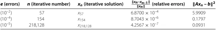
Table 2 x0= (1 1 1 1 1 1 1 1 1 1 1 1 1 1 1 1 1 )T
e(errors) n(iterative number) xn(iterative solution) xn–xn–1xn (relative errors) Axn– b2
(10–2) 57 x
57 6.8700×10⁻⁴ 5.9909
(10–4) 154 x154 8.7043×10⁻⁶ 0.1797
(10–5) 218,128 x218,128 4.2567×10⁻⁷ 0.0931
approximate solution about it. Also, by a series of analyses, we know thatxnis very close to
satisfying the problem ofAx=b. To some extent, we can say that Theorem . solved both (.) andAx=b. Further, as we know, many practical problems in applied sciences such as signal processing and image reconstruction are formulated as the problem ofAx=b. So, our theorem is very useful for solving those problems.
Competing interests
The authors declare that they have no competing interests.
Authors’ contributions
All authors contributed equally to the writing of this paper. All authors read and approved the final manuscript.
Acknowledgements
This work was supported by the Fundamental Research Funds for the Central Universities (3122015L007) and the National Nature Science Foundation of China (11501566).
Received: 30 July 2015 Accepted: 5 October 2015
References
1. Auslender, A: Minimisation de fonctions localement Lipschitziennes: applications a la programmation mi-convexe, mi-differentiable. In: Mangasarian, OL, Meyer, RR, Robinson, SM (eds.) Nonlinear Programming, vol. 3, pp. 429-460. Academic Press, New York (1978)
2. Mahammand, AA, Naseer, S, Xu, HK: Properties and iterative methods for theQ-lasso. Abstr. Appl. Anal.2013, Article ID 250943 (2013)
3. Taheri, S, Mammadov, M, Seifollahi, S: Globally convergent algorithms for solving unconstrained optimization problems. Optimization (2015). doi:10.1080/02331934.2012.745529
4. Xu, HK: Properties and iterative methods for the lasso and its variants. Chin. Ann. Math., Ser. B35(3), 501-518 (2014) 5. Moreau, JJ: Proprietes des applications ‘prox’. C. R. Acad. Sci. Paris, Sér. A Math.256, 1069-1071 (1963)
6. Moreau, JJ: Proximite et dualite dans un espace hilbertien. Bull. Soc. Math. Fr.93, 279-299 (1965)
7. He, SN, Yang, CP: Solving the variational inequality problem defined on intersection of finite level sets. Abstr. Appl. Anal.2013, Article ID 942315 (2013). doi:10.1155/2013/942315
8. Combettes, PL, Wajs, R: Signal recovery by proximal forward-backward splitting. Multiscale Model. Simul.4(4), 1168-1200 (2005)
9. Moudafi, A, Thakur, BS: Solving proximal split feasibility problems without prior knowledge of operator norms. Optim. Lett.8, 2099-2110 (2014)
10. Yao, Z, Cho, SY, Kang, SM, Zhu, LJ: A regularized algorithm for the proximal split feasibility problem. Abstr. Appl. Anal.
2014, Article ID 894272 (2014). doi:10.1155/2014/894272
11. Shehu, Y: Iterative methods for convex proximal split feasibility problems and fixed point problems. Afr. Math. (2015). doi:10.1007/s13370-015-0344-5
12. Shehu, Y, Cai, G, Iyiola, OS: Iterative approximation of solutions for proximal split feasibility problems. Fixed Point Theory Appl.2015, 123 (2015). doi:10.1186/s13663-015-0375-5
13. Shehu, Y, Ogbuisi, FU: Convergence analysis for proximal split feasibility problems and fixed point problems. J. Appl. Math. Comput.48, 221-239 (2015)
14. Duan, PC, He, SN: Generalized viscosity approximation methods for nonexpansive mappings. Fixed Point Theory Appl.2014, 68 (2014). doi:10.1186/1687-1812-2014-68
15. Marino, G, Xu, HK: Weak and strong convergence theorems for strict pseudo-contractions in Hilbert spaces. J. Math. Anal. Appl.329, 336-346 (2007)
16. Xu, HK: Viscosity approximation methods for nonexpansive mappings. J. Math. Anal. Appl.298, 279-291 (2004) 17. Geobel, K, Kirk, WA: Topics in Metric Fixed Point Theory. Cambridge Studies in Advanced Mathematics, vol. 28.
18. Yang, CP, He, SN: General alternative regularization methods for nonexpansive mappings in Hilbert spaces. Fixed Point Theory Appl.2014, 203 (2014)
19. Combettes, PL: Solving monotone inclusions via compositions of nonexpansive averaged operators. Optimization
53, 475-504 (2004)