A Semi Analytic Approach to Coupled Boundary Value Problem

(1)

http://dx.doi.org/10.4236/ajcm.2014.44027

A Semi Analytic Approach to Coupled

Boundary Value Problem

Nityanand P. Pai, Nagaraj N. Katagi

Department of Mathematics, Manipal Institute of Technology, Manipal University, Manipal, India Email: [email protected], [email protected]

This work is licensed under the Creative Commons Attribution International License (CC BY).

http://creativecommons.org/licenses/by/4.0/

Abstract

The present problem is considered as a coupled boundary value problem and is analyzed using a semi analytic method. A series method is used to obtain the solution and region of validity is ex-tended by suitable techniques. In this case of series solution the results obtained are better than pure numerical findings up to moderately large Reynolds numbers. The variation of physical pa-rameters is discussed in detail.

Keywords

Suction, Coupled Equations, Analytic Continuation, Physical Parameters, Reynolds Numbers

1. Introduction

The flow between porous discs has been studied by several authors. As in the case of porous pipes and porous channels, the governing equation reduces to a set of nonlinear ordinary differential equations. This problem was first studied by Batchelor [1] who generalized the solution of Von Karman [2]. Further this problem was ana-lyzed by Stewartson [3] who obtained perturbation solution for the small Reynolds number. Flow between a ro-tating and a stationary disc has been studied by Phan-Thein and Bush [4]. The problem of suction of viscous in incompressible fluid through a rotating porous disc onto a rotating co-axial disc was studied by C. Y. Wang [5]. Here we view this problem as a coupled nonlinear boundary value problem.

In the present paper we have used semianalytical numerical technique to understand the effect of suction represented by a pair of nonlinear differential equations. For simple geometrics the semianalytical numerical methods proposed here provide better results. Van Dyke [6] and his associates have successfully used these se-ries methods in unveiling important features of various types of fluid flows. Bujurke and Pai [7] has discussed similar geometrical problem with injection at the discs.

(2)

phys-ical problem considered in this paper is of great importance in Fluid Dynamics. The present study is a possible extension work of Wang [5]. The problem is solved using a special type of series. The series so generated has limited utility due to presence of a singularity and its region of validity is extended by analytic continuation.

2. Mathematical Formulation

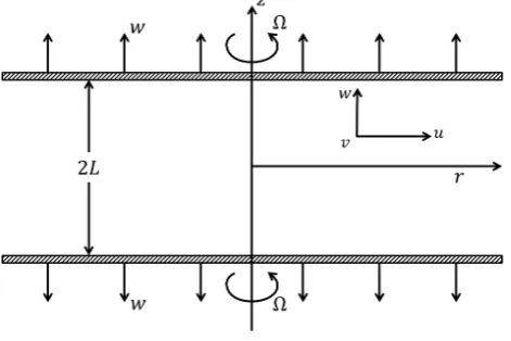
As shown in theFigure 1 we denote the spacing between the discs by z= ±L and rotating with the same an-gular velocity Ω. Fluid is withdrawn from both discs with velocity W. We shall assume the gap with 2L is small compared to diameter of the discs. So that end effects can be neglected. The flow field is symmetric about the

0

z= .

The governing equations are

2

2 2

r

r z

P

v u

uu wu u

r ρ ν r

 

+ − = − + _∇ − _

  (1.1) 2

2

r z

uv v

uv wv v

r ν r

  + + = _∇ − _

  (1.2)

2

z

r z

P

uw ww ν W

ρ

+ = − + ∇ (1.3)

( )

ru r+rwz =0 (1.4)

where

2 2

2

2 2

1

r r

r z

∂ ∂ ∂

∇ = + +

∂

∂ ∂ , and u, v, w are velocity components. The boundary conditions are at z= ±L, 0

u= , v= Ωr , w= ±W .

For similarity transformation we consider Wang [5]

( )

2 2

2 ,

,

2 ,

, 2

W

u rf

L W

v rg

L

w f W

W

p r A P

L η

η

ρ ν η

′ =

= = −

= − +

(1.5)

where z

d

[image:2.595.197.433.551.708.2]

η= and A is constant. Now the equations take the form

(3)

( )

2 2 1 2

f ff g A f

R

′ − ′′− = + ′′′

or

(

)

2R ff′′′ gg′ fiv

− + = (1.6)

(

)

2R f g′ − fg′ =g′′ (1.7)

( )

2 2

2 2 f .

P f W W B

L

η = −_ − ν ′_+

  (1.8)

Here R Wd ν

= is Reynolds number. The boundary conditions are

( )

1

1 0 0 0, 1 ,

2

f′ = f = f′′ = f = − (1.9)

( )

0 0,

( )

1 L .

g g

W β

Ω

′ = = = (1.10)

3. Method of Solution

We assume the solution of (1.6) and (1.7) in the forms

( )

0

( )

1 n

n n

f η f η R f η

∞

=

= +

∑

(3.1)

( )

0

( )

1

.

n n n

g η g η R g η

∞ =

= +

∑

(3.2)

Substituting (3.1), (3.2) in (1.6) and (1.7) and comparing powers of R one can get

1 1

1 2

iv

n r n r r n r

n

f f f g g

∞

− − − −

=

′′′ ′

= −

∑

− (3.3)

(

1 1

)

1

2 0,1, 2 .

n r n r r n r

n

g f f f g n

∞

− − − −

=

′′=

∑

′ − ′ = _ (3.4)

The relevant boundary conditions are

( )

0

( )

0

( )

0

( )

1

1 0, 0 0 0, 1 ,

2

f′ = f = f′′ = f = −

( )

0 0 0, 1 ,

g′ = g =β

( )

1 0,

( )

0 0,

( )

0 0,

( )

1 0,

n n n n

f′ = f = f′′ = f =

( )

1 0 ,

( )

1 0, 1, 2, 3 .

n n

g′ = g = n= 

The solutions are

(

3

)

0 0

1

3 , , 4

f = η − η g =β

(

7 5 2

)

1 1

21 39 19 ,

1120

f = − +η η − η + η

(

4 2

)

1 6 5 ,

8

g =β η η− +

11 9 7 5 3 2 7 5 3

2

1 3 1 177 17 443 137 1 1 13 19

,

560 440 6 140 10 1848 385 840 40 280 840

f =  − η + η − η + η − η − η−β  η − η + η − η

(4)

8 6 4 2 2

3 1 111 253 3183

.

2240 80 3360 560 6720

g =β_ − η + η − η − η + _

 

The slow convergence of series (3.1), (3.2) requires large number of terms for obtaining the approximate sum. For higher order approximations we proceed by the following scheme.

We propose a systematic scheme for this purpose, we consider fn and gn to be of the forms

( )

4 1

(

)

2 , 2 1 n k

n n k

k

f η C η η

+ =

=

∑

− (3.5)

( )

4 ,

(

)

1

1 .

n k

n n k

n

g η D η η

=

∑

− (3.6) We substitute (3.5), (3.6) in (3.3), (3.4) respectively and equate various powers of η on both sides to get

( ) ( ) ( )

₍

₎₍

_{)( )(}

₎

( )( ) ( ) ( )( ) ( )

( ) ( )( )

(

)

( )( ) ( )( ) ( )

(

)

6 3

1 2 1 2 2 1

1 1

2 4 2

7

1 1 2 3 1 3 4

1 0 1 0 1

1 2

2 1 1

2 3 ,

n k n k n k n k i i k i n k i i k i

i i

n nk i nk i

r nk i m t i r nk i t m t i

r i j r j

C C C C P D Q

k K k k

C C P t D D Q t

+ + − + − + − − − − = = − + + + + − − − − − − − − − + = = = = =  = − + ×_ + + + − _    +  − + −    

∑

∑ ∑ ∑



∑ ∑

 (3.7) ( ) ( )

₍

₎

( )( )

(

)

( )( )

(

)

( ) ( )( )

(

)

5 4

1 1 1 1 1

1 1

2 3

6

1 1 3

1 0 1 1

1 1

1

1 , 3 ,

i i

n k n k n k i n k i

i i

n nk i

i nk i m t r i j

D D D T k i C T k i

k k

C D nk i t

+ − + − − + − = = − + + + − − − − = = =  _′ = − _ + − + + − +   + Γ + − − _{− } 

∑

∑∑ ∑

 

(3.8)

where m= −n 4, l=4r+ j, t=4m− j, nk=4n− −2 k, Pi, Qi, Ti’s are functions of k and k1. For the radial velocity profile,

( )

(

)

( )

(

)

(

)

4 1

2 1 1

1 2

1

3 3 2 1 2 .

4

n

n k k k

n k

n k

f η η R C kη k η k η

∞ +

− +

= =

[image:4.595.88.542.130.718.2]

′ = − +

∑ ∑

− − + + + (3.9)

(5)

[image:5.595.142.452.82.379.2]

Table 1. Comparison of values for f′

( )

0 .

R β f′( )0 (numerical) Series method

40.812 3.00 --- –0.34121

20.345 3.6648 –0.54398 –0.54398

0.13151 0.68501 –0.74150 –0.74150

–39.0691 0.98224 -0.6550 –0.65511

–60.000 0.98204 --- –0.41511

Table 2. Comparison of values for f′′′

( )

0 .

R β f′′′( )0 (numerical) Series method

40.812 3.00 --- 0.0000

20.345 3.6648 0.0069 0.00688

8.5679 0.000 0.24870 0.24871

0.13151 0.68501 1.37862 1.37862

–4.39563 0.43440 2.24572 2.24571

–39.0691 0.98224 0.00156 0.00156

–60.000 0.98204 --- 0.00000

And we have

( )

(

) (

)

(

)( )(

)

(

)(

)

2

2 1

4 1

1

1 2 2 1 1

3

2 2 1

n n

n k m

k k k

k

k k k k k k

f η R C η − η − k k kη

∞ +

= =

− − + − + + +

′′′ = +

∑ ∑

− (3.10)

4. Conclusions

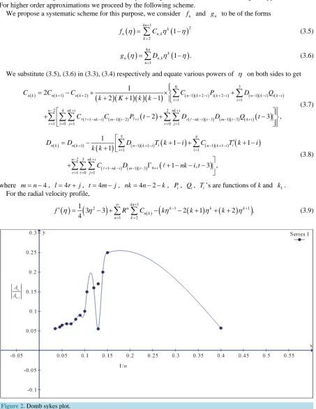
A new type of series is presented for studying the problems of flow between the two discs using recurrences (3.7) and (3.8). In this process we generate universal coefficients Cn k_{( )}, η=1,, 30, k=4n+1.

These coefficients in turn give universal coefficients for fn

( )(

η n=1, 2,, 30

)

. The series (3.9) and (3.10) give f′

( )

0 and f′′′

( )

0 respectively using Domb-sykes plot (Figure 2), and we locate the position of singu-larities for β =0 at 17.89. The series (3.9) and (3.10) are summed using Pade-approximants. Earlier numerical results were from R= 20 to −39. We are able to go upto R= 40 to −60 using Pade-approximants. The results are in close agreement with numerical findings of Wang [5] which are shown in theTable 1 andTable 2.

References

[1] Batchelor, G.K. (1951) Note on Class of Solution of Navier-Stockes Equations Representing Symmetric Flow. Quar-terly Journal of Mechanics Applied Mathematics, 4, 29-35. http://dx.doi.org/10.1093/qjmam/4.1.29

[2] Van Karman, T. (1921) Laminare and Turbulent Reibung. Zeitschrift für Angewandte Mathematik und Mechanik, 1, 233-241. http://dx.doi.org/10.1002/zamm.19210010401

[3] Stewertson, K. (1953) On the Flow between Two Rotating Discs. Proceedings of the Cambridge Philosophical Society, 49, 233-340.

[4] Phan Thein, N. and Bush, M.B. (1984) On the Steady Flow of a Newtonian Fluid between the Parallel Disk. Zeitschrift für Angewandte Mathematik und Physik, 35, 912-919. http://dx.doi.org/10.1007/BF00945453

[5] Wang, C.Y. (1986) Symmetric Viscous Flow between Two Rotating Porous Disc. Quarterly of Applied Mathematics, 4, 29-37.

(6)

[7] Bujurke, N.M. and Pai, N.P. (1995) Computer Extended Series Solution to Viscous Flow between Rotating Discs.

Proceedings of the Indian Academy of Sciences (Mathematical Sciences), 105, 353-369.

http://dx.doi.org/10.1007/BF02837202

(7)