Numerical simulation of one dimensional flood with WENO scheme

(1)

Journal of Chemical and Pharmaceutical Research, 2014, 6(4):265-269

Research Article

ISSN : 0975-7384

CODEN(USA) : JCPRC5

Numerical simulation of one-dimensional flood with WENO scheme

**Y. L. Liu, Y. F. Hong, W. L. Wei* and X. F. Yang**

State Key Laboratory of Eco-Hydraulic Engineering in Shaanxi, Xi’an University of Technology,

Xi’an, Shaanxi, China

_____________________________________________________________________________________________

ABSTRACT

This paper is concerned with a mathematical model for simulating hydrodynamics of 1D flood flows with the WEN O(Weighted Essentially Non-oscillatory Scheme) scheme. The time discretization uses the Runge-Kutta TVD(Total Variation Diminishing) scheme. By using the model, the flow property of dam-break was calculated, and the flow velocity and water depth were obtained. The calculated results show that the WENO scheme has higher accuracy and better stability, and has the ability to automatically capture shock waves, and may suppress the oscillations of numerical solution. This model can effectively simulate the hydrodynamics of 1D river flow.

Keywor ds: WENO scheme; simulation; flood

_____________________________________________________________________________________________

INTRODUCTION

The flood wave caused by a dam fa ilure can result in the loss of hu man lives and has a severe economic impact. Therefore, significant efforts have been carried out over the years to produce methods for determination of the e xtent and timing of the flood wave. Most of these methods are based on the solution of the Shallow Water equations. There are a number of accurate and efficient methods available to solve the Shallow Water equations [1-4].

It is an important basis for validating the numerical method whether the scheme can capture the dam-break bore waves accurately or not. This g ives rise to an increasing interest in solving such a proble m. Fro m 1980 to 2000 several fin ite-difference schemes that handle discontinuities effectively we re used to compute open -channel flo ws, such as the approximate Rie mann solver [3,4]. Based on the above research results, the goal of the current work is to develop a mathe matica l mode l capable of dea ling with hydraulic discontinuities such as steep fronts, hydraulic ju mp and drop, etc. The water governing equations has been solved by the WENO scheme and the Finite Vo lu me Method on unstructured grid.

MATHEMATICAL MODEL

Flow Governing equations

The one-dimensional equations in conservative form in Cartesian coordinates for unsteady gradually va ried flow in open channels are[5].

)

(

)

(

q

b

x

q

f

t

q









(1)



(2)

and q is the conservation physical quantity;

f q

 

is the flu x vector in x direct ion;

b q

 

is the source term vector; h

is flow depth; u is depth-averaged velocity in th e x-d ire ct ion ; g is th e g rav it y acceleration; Sox is the channel

bottom slope in the x-direct ion and is defined as

S

_ox







Z

₀



x

, where Z0 is the bottom elevation; and Sfx is the

friction slope in the x-direction, co mputed using the steady state frict ion formula

S

_fx



（

n

2

u

2



v

2

）

h

4/3, in

which n is the Manning’s roughness coefficient.

Discretization of the flow equation

The integral discretization of Eq. (1) Leads to:





1

1 2 1 2

( )

n n n n

i i i i i

q





q





f q

_



f q

_

 

tb

(2)

in which qn and qn+1 a re the conservation variables for n and n+1 time steps;







t



x

;



t

is t ime step;



x

is

space step; superscript

n

indicates the time layer; subscript

i

denotes space node;

f

_in_₁₂and

f

_i_n₁₂are the nu merical

flux in equation (1).

The key proble m of solution of Eq . (2) is to determine the normal flu x o f

f q

 

. The values of q or

q

may be

discontinuous on the contacting surface of the control volumes, which is a FVM d iscontinuous problem, and brings

difficult ies to the solution off q

 

, and is written asf q

 

 f q q



_L, _R



. The computation of the normal flux

f q

 

has two important aspects: one is the computation of

f q q



_L

,

_R



, the other is the computation of

q

_Land

q

_R( usually is called reconstruction).

Solution of normal fluxes using FDS(Flux Difference Splitting)

The computation of transformation normal fluxes on crossing unit boundary uses Roe’s average FDS method [6]:

 



    

1 2 1 2 1 2 1 2





1 2

L R R L

i i i i

f q  f q_ f q_ a q_ q_ (3)

where the Roe’s speed is



1 2





1 2



1 2 1 2

R L

i i

R L

i i

f q f q

a

q q

 

 

 ,and 1 2

L i

q

_ and

q

_iR__{1 2} are the values of

q

at the left and

right sides of the point

x

_i_₁₂, respectively; thus the normal flu x of the discretization equation (3) may be obtained.

The values of

q

_iL__{1 2}and

q

_iR__{1 2} are obtained by weighting and arraying the stencils with the WENO scheme.

Restructuring of WENO scheme

Now the application of the WENO scheme is explained by the computation of

q

_iL__{1 2} .

The idea used in the WENO schemes is: Given the stencil size k , supposing the k candidate

stencils

S

_r

  

i



x

_{i r}_

,



,

x

_{i r k}_{  }₁



,

r



0 ,



,

k



1

, the k kinds of different restructuring ways may be obtained:

  1

1

2 ₀

k r

rj i r j i

j

q

c q



  





,

r

  

0,

,

k

1

, (4)

Three possible interpolation stencils are:





0 i 2, i 1, i

S  q q q , S1



qi1,q qi, i1



and S2 



q qi, i1,qi2



(3)

i i+1 i+2 i-1

i-2 Stencil 0

Stencil 2

Stencil 1

Fig.1 Ste ncil option of W ENO sche me

The expressions for  ₁

2

r

i

q

_ are:

 0

1 2 1

2

1 7 11

3 i 6 i 6 i

i

q_  q_  q_  q

,  1

1 1 1

2

1

5

1

6

i

6

i

3

i

q

_

 

q

_



q



q

_

,  2

1 1 2

2

1 5 1

3 i 6 i 6 i

i

q_  q  q_  q_

. (5 a, b, c)

The definitions of coefficients are in literature [7].

These optimized schemes for all the k candidate stencils are then convexly co mbined to obtain the W ENO schemes.

The WENO schemes use all the values of  

1 2

r i

q_ to combine convexly to compute 1 2

L i

q

_ .

  1 1 1 2 2 ₀ k _r L r i i r

q



q

  





(6)

in which



_ris the weight.

Determination of Weight



_r

In order to satisfy the stability and the co mpatib ility, we request



r 0and



 



1 0

1

k r r



. Further said that if the

function

q x

 

in all stencils is a smooth function, then the constant

d

_rexists and satisfies:

 





1

2 1

1 1 1

2 ₀ 2 2

k r

L k

r

i i i

r

q

d q

q x

O



  











(7)

After the simple algebraic operation, these coefficients in Eq.(8) may be determined and satisfies

1

1 0





  r k r k

d

.

Under the smooth function situation, we have



_r



d

_r



O





x

k1



,r=0,…,k-1. In order to make the calcu lation

more effectively, we may use the following form the weight





  1 0 k s s r

r







   1 0 k s s r

r





,

r

  

0,

,

k

1

,





2

r r

r d







  , in wh ich



is a rea l nu mber, genera lly ta kes





10

6, to avoid the denominator being

zero.



_k is called “the smooth factor” as a measure of s mooth of the k th possible interpolation reg ion, and its

formula is given in Literature [8](Wei, 2001) .

The third-order mathematical expression for the computation of

q

_iL_{1 2}is:

 0  1  2

1 0 1 1 1 2 1

2 2 2 2

* * *

L

i i i i

q_  q_  q_  q_ (8)

1 2

R i

q

_ is computed by the similar solution method.

(4)

differencing-Time processing

Time processing may use the Rugge-Kutta method with the nature of TVD, for example, regarding the time for mth

order,   1



 



0

i

i k k

ik ik

k

q



q t



L q

 





  ,

i

 

1,

,

m

. At initial time step  0 n

q q , after finishing one

time-step calculation,  m n 1

q q  .

One-Dimensional Dam-Break Simulation

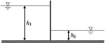
The scenario considered here was the total and instantaneous dam-failure on a flat and frictionless bed. This provides an ideal benchmark test case for shock-capturing schemes since analytica l solution has been known. Figure 2 shows the illustration of the dam-brea k proble m, where the init ial upstream water depth was

h

₁=10 m, and the

[image:4.596.217.396.292.365.2]

downstream water depth was

h

₀=1.The length of the computational region is 200m, and the dam was located at x=200 m. The grid spacing was 1 m. The t ime step was 1 s. Figure 3 shows the water surface position, and Figure 4 shows the velocity distribution, 7.0s after da m fa ilure by using the model, where the solid line represents the analytical solution and the circ le points illustrate the predicted results. It can be seen that the shallower the downstream water depth, then the faster the flood wave travels. The ag ree ment between the analytical and nu merical solutions is satisfactory.

Fig.2 Illustration of the dam -bre ak proble m

Fig. 3 W ate r surface position

Fig. 4 Ve locity distribution

CONCLUSION

(5)

effectively simulate 1D flow acco mpanied with a da m-brea k. The proposed method can a lso be e xpanded to 2D the flows.

Acknowledgments

Partia l financial support of this study from the National Natural Science Foundation of China (Grant No.51178391), Shan xi Province education department funds(2009JK649, 2010JK761)and the special funds for the development of characteristic key d isciplines in the local university supported by the central financia l (Grant No: 00X101, 106-5X1205) and the Shanxi Province key subject construction funds.

REFERENCES

[1]K. Hu, C.G. M ingham, D.M. Causon, Int. J. Numer. Methods in fluids, 1998,28:1241-1261.

DOI:10.1002/(SICI)1097-0363(19981130)28:8<1241:AID-FLD772>3.0.CO;2-2.

[2]K. Anastasiou, C.T. Chan, Int. J . Numer. Methods in fluids, 1997,24:1225-1245. DOI:10.1002/

(SICI)1097-0363(19970615) 24:11<1225:AID-FLD540>3.0.CO;2-D.

[3]C.G. M ingham, D.M . Causon, J. Hydr. Engrg. ASCE, 1998,124:605-614. DOI: 10.1061/

(ASCE)0733-9429(1998)124:6(605).

[4]P. Glaister, Int. J. Numer. Methods in fluids, 1993, 16:629-654. DOI:10.1002/fld.1650160706. [5]Zhao, D.H., J. Water Scientific Advance, 2000, 11:368~373.

[6]P.L. Roe, J. Comp phys, 1981, 43:357-359. DOI:10.1016/0021-9991(81)90128-5.

[7] H.X. Zhang, M.Y. Shen, Computational hydromechanics difference method principle with applications. 2003,Beijing: Defense Industry Publishing House.