Using of Particle Swarm Optimization for Loss Minimization of Vector controlled Induction Motors

(1)

Using of Particle Swarm Optimization for Loss

Minimization of Vector-controlled Induction Motors

Vahid Rashtchi

*

_{, H. Bizhani}

Department of Electrical Engineering, University of Zanjan, Iran

Abstract

This paper presents a new online loss

minimization for an induction motor drive. Among the many loss minimization algorithms (LMAs) for an induction motor, a particle swarm optimization (PSO) has the advantages of fast response and high accuracy. However, the performance of the PSO and other optimization algorithms depend on the accuracy of the modeling of the motor drive and losses. In the development of the loss model, there is always a tradeoff between accuracy and complexity. This paper presents a new online optimization to determine an optimum flux level for the efficiency optimization of the vector-controlled induction motor drive. An induction motor (IM) model in d-q coordinates is referenced to the rotor magnetizing current. This transformation results in no leakage inductance on the rotor side, thus the decomposition into d-q components in the steady-state motor model can be utilized in deriving the motor loss model. The suggested algorithm is simple for implementation.

Keywords

Induction Machine, Loss Minimization,

Magnetizing Current, Particle Swarm Optimization

1. Introduction

More than 50% of the electrical energy produced is consumed by motors, and induction motors are one of the most widely used in electrical drives because of their reliability, ruggedness and relatively low cost. The Induction motors have a high efficiency at rated speed and torque. However, at light loads, motor efficiency decreases drastically due to an imbalance between the copper and the core losses. Electrical motor losses consist of grid loss, converter loss, motor loss and transmission loss. In an effort to improve efficiency, there have been improvements in the materials, design and construction techniques. However, converter loss and motor loss are still greatly dependent on control strategies, especially when the motor operates at light load [1]-[2].

The control strategy to improve motor efficiency can be

divided into two categories: 1) search controller (SC) and 2) loss-model-based controller (LMC). The basic principle of the search controller is to measure the input power and then iteratively search for the flux level (or its equivalent variables) until the minimum input power is detected for a given torque and speed [3]. Important drawbacks of the search controller are the slow convergence and torque ripples. The model-based controller computes losses by using the machine model and selects a flux level that minimizes the losses [4]–[9]. LMC is fast and does not produce torque ripple. However, the accuracy depends on the correct modeling of the motor drive and the losses. Garcia et al. [4] developed a closed-form equation for the optimum flux level in the field-oriented frame. This approach is utilized in an even more simplified form by rearranging the stator resistor [5]. The same approach is utilized by Bernal et al. [6] in deriving a generalized model for the different types of motor. However, in the loss models used in [4]–[6], the leakage inductance is neglected in order to simplify the induction motor equivalent circuit. Lim et al. [7] developed a simplified loss model without sacrificing the leakage inductance, but the developed expression for an optimum flux level has a different format from the one in [4]. Nasir et al. [8] proposed a new online loss-minimization-based algorithm (LMA). In this paper by using the loss model of induction motor and by derived from the power equation, optimum magnetizing current for torque and speed of motor is obtained. In addition, Waheeda et al. [9] by using the loss model introduced in [8] and genetic algorithm, optimized the current magnetizing of induction motor to improve the efficiency.

(2)

balance between copper and iron losses is achieved to minimize the electromagnetic losses.

The ideal loss model will be an accurate and simple one. In this paper, an induction motor model with an iron loss resistor is referenced to the rotor magnetizing current, thus no leakage inductance is considered on the rotor side. Based on this model, we can derive the equation to find an optimum flux level in the same fashion as the one in [4], which is widely used for the development of the LMA, without neglecting leakage inductance. The performance of the proposed optimization algorithm is tested in simulation at different operation conditions. The result show that the performance of the drive with PSO algorithm is improved in terms of power saving and fast responding as compared to without optimization and other optimization algorithm such as LMA and GA.

2. Induction Motor and Loss Model

According to the literatures there are two approaches of modeling of IM taking in to account the iron loss, namely parallel and series iron loss model. Even though the series model has less number of differential equations, a parallel model is superior than the other one [9].

In this section we present the induction motor model and this loss model respectively.

Induction Motor Model

An equivalent circuit for IM can be varied by the different choices of flux linkage constants [8]. In this paper, we utilize an equivalent circuit referenced to the rotor magnetizing current by defining the rotor flux as 𝜓𝜓𝑟𝑟=𝐿𝐿𝑚𝑚𝑖𝑖𝑚𝑚𝑟𝑟. The

notion for this transformation is illustrated in Fig. 1. An iron loss resistor 𝑅𝑅𝑓𝑓′ is added in parallel to the magnetizing

inductance in a reference frame fixed to the rotor magnetizing current, and the d-axis has been aligned in the direction of the magnetizing current 𝑖𝑖𝑚𝑚𝑟𝑟 as shown in Figs. 2

and 3. Defining the differential operator 𝑝𝑝 ≡ 𝑑𝑑/𝑑𝑑𝑑𝑑, the space vector motor model in a rotating reference frame is

given by (1)–(2), where 𝜔𝜔𝑒𝑒=𝑑𝑑𝜃𝜃𝑒𝑒/𝑑𝑑𝑑𝑑 is the electrical

angular speed of the rotor and 𝜔𝜔𝑟𝑟=𝑑𝑑𝜃𝜃𝑟𝑟/𝑑𝑑𝑑𝑑 is the electrical

rotor speed.

m m e m m s s e s s s s

s

R

i

pL

i

j

L

i

pL

i

j

L

i

u

=

+

'

+

ω

'

+

'

+

ω

'

₍₁₎

(

)( ' / ' )

(

))( ' / ' )

s m f r m e m f m e r m r m

i i i i i

p j

L

R i

p j

L

R i

ω

ω ω

= + + = +

+

[image:2.595.313.554.109.349.2]

+ +

−

₍₂₎

Figure 1. Phasor diagram of steady-state equivalent circuits of an

induction motor [8].

Figure 2. Phasor diagram of equivalent circuit and rotor field angle

definition [8].

[image:2.595.314.548.388.523.2] [image:2.595.137.479.567.722.2]

(3)

Using 𝑢𝑢𝑠𝑠=𝑢𝑢𝑠𝑠𝑠𝑠+𝑗𝑗𝑢𝑢𝑠𝑠𝑠𝑠 , 𝑖𝑖𝑠𝑠=𝑖𝑖𝑠𝑠𝑠𝑠+𝑗𝑗𝑖𝑖𝑠𝑠𝑠𝑠 , 𝑖𝑖𝑚𝑚=𝑖𝑖𝑚𝑚𝑠𝑠+

𝑗𝑗𝑖𝑖𝑚𝑚𝑠𝑠 and 𝑖𝑖𝑚𝑚𝑠𝑠 = 0 , 𝑖𝑖𝑚𝑚𝑠𝑠 =𝑖𝑖𝑚𝑚𝑟𝑟 =𝑐𝑐𝑐𝑐𝑐𝑐𝑐𝑐𝑑𝑑𝑐𝑐𝑐𝑐𝑑𝑑 for

rotor-flux-orientation control scheme, we obtain from (1)-(2) that mr m sq s e sd s sd s

sd

R

i

pL

i

L

i

pL

i

u

=

+

'

−

ω

'

+

'

(3)

mr m e sd s e sq s sq s

sq

R

i

pL

i

L

i

L

i

u

=

+

'

+

ω

'

+

ω

'

(4)

mr r m f m mr

sd

i

p

L

R

L

R

i

=

+

(

'

/

'

+

'

/

'

)

(5)

mr r m r e mr f m e

sq

L

R

i

L

R

i

=

ω

(

'

/

'

)

+

(

ω

−

ω

)(

'

/

'

)

(6) Let 𝑅𝑅𝑡𝑡=𝑅𝑅𝑓𝑓′ ∥ 𝑅𝑅𝑟𝑟′, from (3) the magnetizing current can

be expressed by:

1/ (1

( ' / '

' / ' ))

1/ (1

' / ' )

mr m r m f sd m t sd

i

p L

R

L

R

i

pL

R i

=

+

=

+

(7)

From (6), the slip speed can be derived as:

( ' / ' ) /

' / '

( ' / ' ) /

' / '

slip r m sq mr e r f t m sq mr r t f

R L i i

R R

R L i i

R R

ω

=

−

=

−

(8)

In the steady state of this motor model, there is no leakage inductance on the rotor side and the sum of the recalculated rotor current 𝑖𝑖𝑟𝑟 and the iron current 𝑖𝑖𝑓𝑓 is perpendicular to

the magnetizing current 𝑖𝑖𝑚𝑚𝑟𝑟. Because of this, the circuit

illustrates decomposition of the stator current 𝑖𝑖𝑠𝑠 into the

rotor flux-oriented components: 𝑖𝑖𝑠𝑠𝑠𝑠=𝑖𝑖𝑚𝑚𝑟𝑟 which forms the

flux 𝜓𝜓𝑟𝑟, and 𝑖𝑖𝑠𝑠𝑠𝑠=𝑖𝑖𝑓𝑓+𝑖𝑖𝑟𝑟 which is related to the control of

torque developed by the motor. Note that due to the existence of 𝑖𝑖𝑓𝑓, 𝑖𝑖𝑟𝑟 controls the torque. From the motor model (3)–(6),

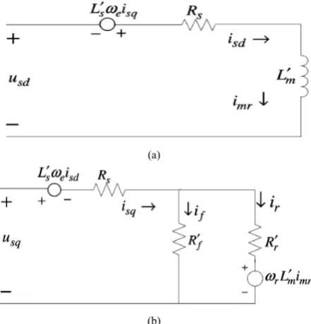
the steady-state IM equivalent circuit in a field-oriented frame can be shown as in Fig. 4. Fig. 4(a) can easily be derived from (3) and (5) and Fig. 4(b) can easily be derived from (4) and (6) considering that the terms with differentiation will be zero in steady state [8].

(a)

(b)

Figure 4. Steady-state IM equivalent circuit in: (a) d-axis and (b) q-axis

[8].

Loss Model

[image:3.595.68.289.490.720.2]

In the development of the loss model, a typical method for model simplicity used in previous research is to ignore the leakage inductance. The decomposition feature of the proposed motor model makes the derivation of the loss model more straightforward without any assumption for model simplicity. Stator copper, rotor copper and iron losses dominate the overall power loss compared to stray, friction, windage, and converter losses [8]. In the current work, stray, friction, windage, and converter losses are neglected. From Fig. 4, the total loss is given by:

2 2 2 2

(

)

' (

)

'

total cu iron cur

s sd sq f sq r r r

P

R i

i

R i

i

R i

=

+

=

+

−

+

(9)

Where 𝑃𝑃𝑐𝑐𝑐𝑐𝑠𝑠 is stator copper losses, 𝑃𝑃𝑖𝑖𝑟𝑟𝑖𝑖𝑖𝑖 is iron losses

and 𝑃𝑃𝑐𝑐𝑐𝑐𝑟𝑟 : is rotor copper losses. Since only the stator

voltage and the current are real state variables, we need to express the total losses in terms of 𝑖𝑖𝑠𝑠𝑠𝑠 and 𝑖𝑖𝑠𝑠𝑠𝑠.

From Fig. 4, the rotor current can be expressed as:

( ' / ' )

( ' / ( '

' ))

( ' / ( '

' ))

r sq f sq r f r r m f sd

f f r sq r m f r sd

i i

i

R R i

L

R i

R

i

L

R

i

ω

=

− =

−

=

+

−

+

(10)

Substituting 𝑖𝑖𝑟𝑟from (10) into (9) yields:

,

2 2 sq q sd d

total

R

i

R

i

P

=

+

,

))

'

/(

'

(

m2 f r r2 s

d

R

L

R

=

+

ω

)

'

/(

'

_f _r _f _r s

q

R

=

+

(11)

The developed electrical torque can be expressed in different ways. From Fig. 4 and (10), one can express the torque as:

2

(3/ 2)

'

(3/ 2)

' ( ' / ( '

' ))

(3/ 2) ( '

) / ( '

' )

e P m mr r P m r f r sq mr

P m mr f r r

T

Z L i i

Z L R

R

R i i

Z L i

R

ω

=

+

−

+

(12) By utilizing (8), torque can also be written as:

2

(3 / 2) ( '

) / '

(3 / 2)

'

(3 / 2) (( '

) / ' )

e P m mr r slip

P m mr sq P m mr f e

T

Z L i

R

Z L i i

Z L i

R

ω

=

−

(13) If the second expression from (8) is used in (13), the torque expression (13) becomes the same as (12). The second term of the right side of (13) represents the loss in developed torque due to iron loss resistance. Since 𝑅𝑅′𝑓𝑓 ≫ 𝑅𝑅𝑟𝑟′ and

(𝑅𝑅′𝑓𝑓+𝑅𝑅𝑟𝑟′)≫(𝐿𝐿′𝑚𝑚𝑖𝑖𝑚𝑚𝑟𝑟)2 , torque (12)–(13) can be

approximated as: mr sq t mr sq m P

e

Z

L

i

K

i

T

≈

(

3 /

2 )

'

=

(14)

Where, 𝐾𝐾𝑡𝑡= (3/2)𝑍𝑍𝑝𝑝𝐿𝐿′𝑚𝑚.

Then in the steady state 𝑖𝑖𝑠𝑠𝑠𝑠=𝑇𝑇𝑇𝑇/(𝐾𝐾𝑡𝑡𝑖𝑖𝑚𝑚𝑟𝑟) and 𝑖𝑖𝑠𝑠𝑠𝑠=𝑖𝑖𝑚𝑚𝑟𝑟.

Thus the total loss in the steady state can be written in terms of magnetizing current 𝑖𝑖𝑚𝑚𝑟𝑟 [8].

2 2

₍

_/(

₎₎

mr t e q mr d

total

R

i

R

T

K

i

(4)

[image:4.595.115.494.86.338.2]

Figure 5. Block diagram of proposed loss minimization scheme for IM

3. Mechanism of Loss Minimization

The iron loss can be minimized by using a minimum possible field flux corresponding to a given torque and motor speed. The stator copper loss component due to the magnetizing current is consequently minimized. The flux can be reduced by decreasing the flux component current 𝑖𝑖𝑚𝑚𝑟𝑟 . Because under vector control condition, the

electromagnetic torque produced is proportional to the product of the rotor flux and torque component of the stator current 𝑖𝑖𝑠𝑠𝑠𝑠, in order to maintain the same torque with

reduced rotor flux, this torque component of stator current must be increased. By a proper adjustment of the magnetic flux, an appropriate balance between copper and iron losses can be achieved to minimize the electromagnetic losses.

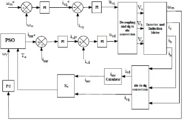
Block Diagram of the Proposed System

A simplified block diagram of the proposed optimization method is shown in Fig. 5; it is implemented in a classical rotor flux oriented control (FOC). In this scheme two phase currents are measured in order to calculate the electromagnetic torque. The torque and the speed are the parameters used by the particle swarm optimization algorithm to minimize the objective function which is the total loss of the motor (15). PSO algorithm output is a reference value of magnetizing current (which corresponds to minimum loss for the given torque and speed) to the motor.

PSO Algorithm Procedure

Some evolutionary optimization algorithms like GA, ICA, honey bee algorithm [10]-[11] are presented for optimization of complicated fitness functions.

This optimization procedure consists of searching the optimum magnetizing current (flux) value for a given torque and speed relying on PSO algorithm, [12]. PSO is an efficient algorithm for population-based optimization invented by Kennedy and Eberhart (1995) and further developed in recent years. It is inspired by the social behavior of animals, e.g. bird flocking or fish schooling. Compared with other optimization algorithms, PSO is particularly well suited to complex optimization problems, with faster convergence rate. An additional advantage is that PSO requires fewer parameters for regulation than other optimization algorithms. In PSO, a “particle”, located at any point in D-dimensional search space, represents a potential solution to the optimization problem.

1) Possible Topologies of PSO:

 Star topology: In this topology each particle can communicates with members of swarm and each particle tends to flow global best of population. This topology is used in global best algorithm.

 Ring topology: In this topology each particle communicates with N neighbor particles and each particle tends to follow movement of best particle among neighbor particles. This topology is used in local best algorithm.

(5)

These topologies are shown in Figs. 6.

(a) (b) (c)

Figure 6. Topologies of PSO: a) Star topology b) Ring Topology c) Wheel

Topology

Types of PSO Algorithm

Based on these topologies three type of algorithm have been developed, which are as follows:

 Individual best: This algorithm is based on wheel topology and is similar to one group of climbers that are not connected to each other and move based on self-experiences along their paths.

 Local best: this algorithm uses ring topology, so that particles are affected by best particle in neighbor region.

 Global best: This algorithm applies star topology. Movement of each particle is based on self-experiences and movement of other particles. Movement of particles completely depend on other particle's movement.

Since in the present work global best method is used, this method is briefly described in the next section.

2) Global Best Method

Implementation steps of this algorithm are as follows [12]: 1-Random generating of primary population,

2-Particles fitness calculation respect to their current position.

3-Comparsion current fitness of particles with their best experience:

𝑖𝑖𝑖𝑖:𝐹𝐹(𝑃𝑃𝑖𝑖) >𝑝𝑝𝑝𝑝𝑇𝑇𝑐𝑐𝑑𝑑𝑖𝑖

𝑑𝑑ℎ𝑇𝑇𝑐𝑐𝑝𝑝𝑝𝑝𝑇𝑇𝑐𝑐𝑑𝑑𝑖𝑖=𝐹𝐹(𝑃𝑃𝑖𝑖), ��𝑥𝑥𝑝𝑝𝑝𝑝𝑇𝑇𝑐𝑐𝑑𝑑𝚤𝚤=𝑥𝑥�𝚤𝚤(𝑑𝑑)

4-Comparsion of the current fitness of particles with the best experience of all particles:

𝑖𝑖𝑖𝑖:𝐹𝐹(𝑃𝑃𝑖𝑖) >𝑔𝑔𝑝𝑝𝑇𝑇𝑐𝑐t

𝑑𝑑ℎ𝑇𝑇𝑐𝑐𝑔𝑔𝑝𝑝𝑇𝑇𝑐𝑐t =𝐹𝐹(𝑃𝑃𝑖𝑖), ��𝑥𝑥𝑔𝑔𝑝𝑝𝑇𝑇𝑐𝑐t=𝑥𝑥�𝚤𝚤(𝑑𝑑)

5-Change in velocity of each particle according to (16):

))

(

))

(

)

1 (

)

(

t

v

t

r

1

c

1

xpbest

x

t

r

2

c

2

xgbest

x

t

v

i

=

i

−

+

i

−

i

+

−

i

(16) 6-The particle position change to new position according to (17):

)

(

)

1 (

)

(

t

x

t

v

t

x

_i

=

_i

−

+

_i (17)

7- Algorithm is iterated from step 2 until the convergence is obtained.

4. Simulation Results

[image:5.595.59.297.77.194.2]

The simulation of efficiency optimization of induction motor using particle swarm optimization algorithm is performed by using Matlab/simulink software, the results of different cases are given below. The induction machine parameters are shown in TABLE 1. The aim to use the optimization algorithm is to let the motor work at variable flux to minimize the loss and hence optimize efficiency, also to prove the effectiveness and the robustness of the proposed algorithm the motor drive was tested at different range of speeds.

Table 1. Induction Motor and PSO Data Used For Simulation

Parameter Value

Power 9 kW

Voltage 460 V

Stator resistance 0.399Ω

Referred rotor resistance 0.3107Ω Referred iron loss resistance 570.7Ω

Number of pole pair 2

Referred stator inductance 6.3mH Referred mutual inductance 53mH Inertia constant 0.05 kgm2

Rated speed 1750 rev/min

Friction coefficient 0.0006

Frequency 60Hz

Inertia Weight 1

Personal Learning Coefficient

(c1) 1

Global Learning Coefficient (c2) 1

Using the PSO algorithm in MATLAB, loss equation (15) is minimized to obtain the value of reference magnetizing current. Simulation is done for different speeds and torques and loss is found to be reduced very much and efficiency is improved at light loads with PSO algorithm.

Simulation is carried out for a speed of 180rad/s and a torque of 5Nm. Using PSO algorithm the magnetizing current obtained is 5.98A and this reference value is applied to the motor for loss minimization (See Fig. 10).

When the magnetizing current is reduced to 5.98A, there will be corresponding reduction in flux level and thus core loss is reduced. But to meet the torque, according to equation (14) there should be corresponding increase in q-axis stator current. Then the copper loss is increased. The maximum efficiency will be obtained for the motor when core loss equals copper loss.

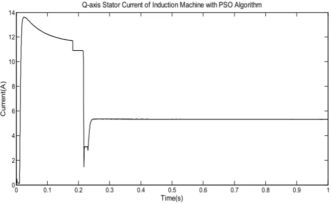
[image:5.595.311.552.292.532.2]

(6)

show the speed, torque, three phase stator currents, magnetizing current and q-axis stator current respectively. The results show that by using PSO algorithm for optimization of magnetizing current, performance of

induction machine do not change. However, efficiency of motor improves in this optimization. At steady state since 𝑖𝑖𝑠𝑠𝑠𝑠=𝑖𝑖𝑚𝑚𝑟𝑟, the magnetizing current is minimized to 5.98A

corresponding to the given torque and speed.

Figure 7. Speed of induction motor with PSO algorithm

Figure 8. Torque of induction motor with PSO algorithm

Figure 9. Three phase currents of induction motor with PSO algorithm

0 0.1 0.2 0.3 0.4 0.5 0.6 0.7 0.8 0.9 1

-50 0 50 100 150 200

Time(s)

S

peed(

rad/

s)

Speed of Induction motor with PSO algorithm

0 0.1 0.2 0.3 0.4 0.5 0.6 0.7 0.8 0.9 1

0 5 10 15 20 25 30 35 40

Time(s)

Tor

que(

N

.M

)

Torque of Induction Motor with PSO Algorithm

0 0.1 0.2 0.3 0.4 0.5 0.6 0.7 0.8 0.9 1

-250 -200 -150 -100 -50 0 50 100 150 200 250

Time(s)

C

urre

nt

(A

)

[image:6.595.134.476.127.730.2]

(7)

[image:7.595.138.473.81.271.2]

Figure 10. Optimum magnetizing current of induction machine with PSO algorithm

Figure 11. Q-axis current of induction machine with PSO algorithm

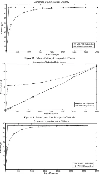
Simulations are done for speeds 157rad/s and 100rad/s with different load torques with and without optimization. Efficiency vs output power and power loss vs output power are plotted for the above two cases. In both cases the maximum efficiency is almost same. Figs. 12 and 13, represent the efficiency and power loss with and without PSO at 100rad/s and Figs.14 and 15, represent the efficiency and power loss with and without PSO at 157rad/s.

Figs. 12 and 14 show that there is great efficiency improvement at light loads when using PSO procedure. Thus large amount of energy saving can be done using this method.

0 0.1 0.2 0.3 0.4 0.5 0.6 0.7 0.8 0.9 1

0 2 4 6 8 10 12 14 16 18

Time(s)

C

urre

nt

(A

)

Optimum Magnetizing Current of Induction Machine with PSO Algorithm

0 0.1 0.2 0.3 0.4 0.5 0.6 0.7 0.8 0.9 1

0 2 4 6 8 10 12 14

Time(s)

C

urre

nt

(A

)

[image:7.595.138.472.298.503.2]

(8)

Figure 12. Motor efficiency for a speed of 100rad/s

[image:8.595.137.475.73.669.2]

Figure 13. Motor power loss for a speed of 100rad/s

Figure 14. Motor efficiency for a speed of 157rad/s

0 500 1000 1500 2000 2500 3000 3500 4000

0 10 20 30 40 50 60 70 80 90 100

Output Power(w)

E

ffi

ci

en

cy(

%

)

Comparsion of Induction Motor Efficiency

With PSO Optimization Without Optimization

0 500 1000 1500 2000 2500 3000 3500 4000

0 50 100 150 200 250 300

Output Power(w)

P

ow

er

Los

s(

w

)

Comparsion of Induction Motor Losses

With PSO Algorithm Without Optimization

0 1000 2000 3000 4000 5000 6000 7000

0 10 20 30 40 50 60 70 80 90 100

Output Power(w)

E

ffi

ci

en

cy(

%

)

Comparsion of Induction Motor Efficiency

(9)

[image:9.595.135.476.80.276.2]

Figure 15. Motor power loss for a speed of 157rad/s

Table 2. Comparsion of Induction Machine Parameters in PSO Procedure and Without Optimization

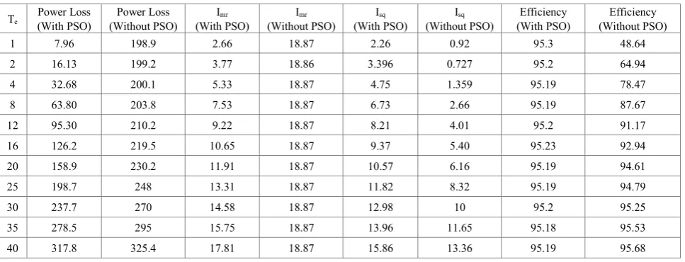
Te Power Loss _{(With PSO)} _{(Without PSO)}Power Loss _{(With PSO)}Imr _{(Without PSO)}Imr _{(With PSO)}Isq _{(Without PSO)}Isq _{(With PSO)}Efficiency _{(Without PSO)}Efficiency

1 7.96 198.9 2.66 18.87 2.26 0.92 95.3 48.64

2 16.13 199.2 3.77 18.86 3.396 0.727 95.2 64.94

4 32.68 200.1 5.33 18.87 4.75 1.359 95.19 78.47

8 63.80 203.8 7.53 18.87 6.73 2.66 95.19 87.67

12 95.30 210.2 9.22 18.87 8.21 4.01 95.2 91.17

16 126.2 219.5 10.65 18.87 9.37 5.40 95.23 92.94

20 158.9 230.2 11.91 18.87 10.57 6.16 95.19 94.61

25 198.7 248 13.31 18.87 11.82 8.32 95.19 94.79

30 237.7 270 14.58 18.87 12.98 10 95.2 95.25

35 278.5 295 15.75 18.87 13.96 11.65 95.18 95.53

40 317.8 325.4 17.81 18.87 15.86 13.36 95.19 95.68

Furthermore other simulations are done for comparsion of values of the magnetizing current 𝑖𝑖𝑚𝑚𝑟𝑟, q-axis stator current

𝑖𝑖𝑠𝑠𝑠𝑠 and efficiency for different load torques at a constant

speed of 180 rad/s for with PSO algorithm and without optimization (See Table. 2). From this, it can be seen in simulation with PSO algorithm when the load torque is increased, value of 𝑖𝑖𝑚𝑚𝑟𝑟 (optimum value) at minimum loss

condition also increased. Since 𝑖𝑖𝑠𝑠𝑠𝑠 increasing, the required

torque is developed to meet the torque demand. Nevertheless in simulation without optimization values of magnetizing current are constant.

When load torque is nearer or at rated value, the reference magnetizing current is at rated value, too. Thus the flux of the machine will be at rated value at rated condition. So the machine can easily run at rated load torque without any torque capability problem. Motor efficiency is almost constant at all loads and it is 95%.

5. Conclusions

A new online loss-minimization algorithm based on PSO

algorithm is proposed and simulated for vector controlled induction motor drive. The advantages of using PSO have been highlighted. Maximum efficiency is obtained for all speeds ranges and torques, because with PSO global optimum is more probable. Extensive simulation results of proposed optimization method and FOC method without optimization are investigated and compared and the superiority of the former is confirmed. It appears that non negligible energy can be saved with the use of PSO.

Nomenclature

𝑅𝑅𝑠𝑠 ,𝑅𝑅𝑟𝑟 Resistances of the stator and rotor phase

winding.

𝐿𝐿𝑠𝑠 ,𝐿𝐿𝑟𝑟 Self-inductances of the stator and the rotor.

𝐿𝐿𝑚𝑚 Magnetizing inductance.

𝑅𝑅′𝑟𝑟 Referred rotor resistance.

𝑅𝑅𝑓𝑓′ Referred iron-loss resistance

𝐿𝐿𝑠𝑠′ , 𝐿𝐿′𝑚𝑚 Referred stator and magnetizing inductances.

𝑍𝑍𝑝𝑝 Stator voltages complex space vector.

0 1000 2000 3000 4000 5000 6000 7000

0 50 100 150 200 250 300 350

Output Power(w)

P

ow

er

Los

s(

w

)

Comparsion of Induction Motor Losses

[image:9.595.65.549.308.493.2]

(10)

𝑢𝑢𝑠𝑠 ,𝑖𝑖𝑠𝑠 Stator voltage and current complex space

vectors.

𝜔𝜔𝑒𝑒 Angular speed of the rotor flux.

𝜔𝜔𝑟𝑟 Electrical rotor speed.

𝜔𝜔𝑚𝑚 Mechanical rotor speed.

𝜃𝜃 Rotor flux angle. 𝐹𝐹(𝑃𝑃𝑖𝑖) Fitness of i-th particle

𝑥𝑥�𝚤𝚤(𝑑𝑑) Position of the i-th particle

𝑝𝑝𝑝𝑝𝑇𝑇𝑐𝑐𝑑𝑑𝑖𝑖 Best fitness of i-th particle

𝑥𝑥𝑝𝑝𝑝𝑝𝑇𝑇𝑐𝑐𝑑𝑑𝚤𝚤

�� _{Position of the i-th particle related to}_{𝑝𝑝𝑝𝑝𝑇𝑇𝑐𝑐𝑑𝑑}_𝑖𝑖 𝑔𝑔𝑝𝑝𝑇𝑇𝑐𝑐𝑑𝑑 Best fitness of all particles in the population 𝑥𝑥𝑔𝑔𝑝𝑝𝑇𝑇𝑐𝑐𝑑𝑑

�� _{Position of the particle with the best fitness} 𝑟𝑟1 ,𝑟𝑟2 Random numbers in (0,1) distance

𝑐𝑐1 ,𝑐𝑐2 Acceleration coefficients

REFERENCES

[1] J. Malinowski, J. McCormick, and K. Dunn, “Advances in

construction techniques of AC induction motors: Preparation for super-premium efficiency levels,” IEEE Trans. Ind. Appl., vol. 40, no. 6, pp. 1665–1670, Nov-Dec 2004.

[2] J. L. Kirtley, J. Cowie, E. F. Brush, D. T. Peters, and R. Kimmich, “Improving induction motor efficiency with Die-cast copper rotor cages,” in Proc. PES General Meeting, 2007, pp. 1–6.

[3] D. S. Kirschen, D. W. Novotny, and T. A. Lipo, “On-line efficiency optimization of a variable frequency induction motor drive,” IEEE Trans. Ind. Appl., vol. IA-21, no. 4, pp. 610–616, May/Jun. 1985.

[4] G. O. Garcia, J. C. Mendes Luis, R. M. Stephan, and E. H. Watanabe, “An efficient controller for an adjustable speed

induction motor drive,” IEEE Trans. Ind. Electron., vol. 41, no. 5, pp. 535–539, Oct. 1994.

[5] C. Chakraborty and Y. Hori, “Fast efficiency optimization techniques for the indirect vector-controlled induction motor drives,” IEEE Trans. Ind. Appl., vol. 39, no. 4, pp. 1070–1076, Jul./Aug. 2003.

[6] F. Fernandez-Bernal, A. Garcia-Cerrada, and R. Faure,

“Model-based loss minimization for DC and AC Vector-Controlled Motors Including Core Saturation,” IEEE Trans. Ind. Appl., vol. 36, no. 3, pp. 755–763, May/Jun. 2000.

[7] S. Lim and K. Nam, “Loss-minimising control scheme for

induction motors,” Proc. Inst. Elect. Eng., vol. 151, no. 4, pp. 385–397, Jul. 2004.

[8] M. Nasir Uddin, and Sang Woo Nam, “New Online Loss-

Minimization Based Control of an Induction Motor Drive,”

IEEE Transactions on Power Electronics, vol. 23, no. 2, pp. 926-933, March 2008.

[9] M. Waheeda, A. Sureshkumar and H. S. Sibin, “Loss

minimization of Vector Controlled Induction Motor Drive

using Genetic Algorithm,” International Conference on

Green Technologies (ICGT), pp. 251-257, Dec. 2012.

[10] V. Rashtchi, E. Rahimpour and H.Shahrouzi,”Model

reduction of transformer detailed R-C-L-M model using the imperialist competitive algorithm” IET Electric Power Applications, Vol 6, Issue 4, pp. 233-242, April 2012. [11] V.Rashtchi, J.Gholinezhad, P.Farhang, “Optimal coordination

of overcurrent relays using Honey Bee Algorithm”, International Congress on Ultra Modern Telecommunications and Control Systems and Workshops, ICUMT 2010, pp.401-405