Ab initio quasiharmonic equations of state for dynamically stabilized soft-mode materials
N. D. Drummond and G. J. Ackland
Department of Physics and Astronomy, The University of Edinburgh, JCMB, The King’s Buildings, Edinburgh, United Kingdom 共Received 29 October 2001; revised manuscript received 30 January 2002; published 25 April 2002兲
We introduce a method for treating soft modes within the analytical framework of the quasiharmonic equation of state. The corresponding double-well energy-displacement relation is fitted to a functional form that is harmonic in both the low- and high-energy limits. Using density-functional calculations and statistical physics, we apply the quasiharmonic methodology to solid periclase 共MgO兲. We predict the existence of a
B1-B2 phase transition at high pressures and temperatures.
DOI: 10.1103/PhysRevB.65.184104 PACS number共s兲: 61.50.Ks, 64.70.Kb, 71.20.⫺b
I. INTRODUCTION
The quasiharmonic approximation1 provides a means of extracting finite-temperature properties of materials from static calculations. It assumes that the vibrational properties can be understood in terms of excitations of noninteracting harmonic normal modes: phonons. Lattice dynamics2can be used to calculate phonon energies by evaluating the eigen-values of the dynamical matrix, which involves second de-rivatives of the crystal energy with respect to atomic dis-placements.
The frequencies of these modes depend on the crystal’s density. Hence they have a temperature dependence that arises simply because of thermal expansion in the material.
Recent developments in ab initio energy calculations have enabled full phonon dispersion curves to be obtained, leading to a resurgence of interest in the quasiharmonic approach. Difficulties arise, however, when the dynamical matrix has negative eigenvalues, indicating that the crystallographic structure is not a local minimum of energy. Such crystals may be dynamically stabilized: because of their large en-tropy, they may represent a minimum of free energy at high temperature. Within the conventional assumption of har-monic phonons, the quasiharhar-monic framework leads to diver-gent free energies in these cases. Such systems have been treated numerically from first principles using Monte Carlo methods with effective Hamiltonians3 or molecular-dynamics simulations of a reduced set of modes.4 Here we relax the quasiharmonic assumption of harmonic modes while retaining the approximation of noninteracting phonons, and show how the intrinsic anharmonicity of such modes can be included in analytic free-energy calculations.
The mineral periclase 共MgO兲 is of some geological sig-nificance as one of the supposed constituents of the Earth’s lower mantle. It is generally believed that along the geotherm—the conditions of pressure and temperature actu-ally occurring in the mantle—periclase remains in a single phase. Under other conditions, however, previous calcula-tions have suggested that periclase has two phases in its solid state: a sodium chloride-like face-centered-cubic phase (B1) and a cesium chloride-like simple cubic phase (B2) that is favored at extremely high pressures.5
Imaginary phonon frequencies are found in the B2 phase of periclase, and have attracted enormous attention in the other principal constituent of the lower mantle, magnesium
silicate perovskite (MgSiO3).6 –10 Equilibrium structures, thermodynamic properties, and compositions depend on the free energy. Here we present a calculation of the free energy of periclase as a function of density and temperature. We use the pseudopotential-plane-wave approach to evaluate total energies and the method of finite displacements to evaluate pressure-dependent force constants,11 including effective charges and dielectric constants12 for the longitudinal optic modes. Based on calculated phonon frequencies and the quasiharmonic approximation, we present a first-principles calculation of the phase diagram and thermodynamic equa-tion of state of solid periclase: the relaequa-tionship between pres-sure, density, and temperature.
II. QUASIHARMONIC METHOD
A. Ab initio calculation of specific Helmholtz free energies
The first stage of the calculation is to obtain the specific 共with respect to mass兲Helmholtz free energy of each phase as a function of density and temperature. We write the free energy as the sum of the frozen-ion interaction energy and the free energy due to lattice vibrations.
1. Frozen-ion energy
The frozen-ion energy—the interaction energy of the crystal with the ions fixed in their equilibrium positions—is, by definition, temperature independent. Hence the free en-ergy is simply equal to the internal enen-ergy. In order to deter-mine the dependence on density, total-energy density-functional calculations are carried out for each phase at a range of different lattice parameters.
2. Lattice thermal Helmholtz free energy
We calculate the lattice thermal Helmholtz free energy of each phase as a function of density and temperature within the framework of the harmonic approximation.13
We denote the matrix of force constants by , where l,n,␣;m, p,is the component of force in direction␣ on ion n in unit cell l when ion p in unit cell m is displaced infinitesi-mally in direction , divided by the magnitude of the dis-placement.
Pairs of density-functional calculations are carried out with an ion displaced from equilibrium along one of the Cartesian axes by a small amount in first a positive sense and then a negative sense. By averaging the resulting Hellmann-Feynman forces on the ions from the first simulation with the negative of the forces from the second, first-order anhar-monic contributions to the force constants are eliminated.
The set of rotations under which the crystal structure is invariant are identified and the rotation matrices, together with the mappings between the ions under the symmetry operations, are evaluated. For a given pair of ions (l,n) and (m, p), the matrix of force constantsl,n,␣;m, p, transforms as a second-rank tensor. However, for a symmetry operation, the transformed matrix must be the same as the 共unrotated兲 matrix of force constants between the pair of ions which are mapped to (l,n) and (m, p). Hence new elements of the matrix of force constants can be obtained by an application of these point symmetries. Translational symmetries can be identified and exploited in a similar fashion.
The matrix of force constants should be symmetric,13and Newton’s third law must be satisfied: if an ion is displaced slightly then the restoring force on that ion must be equal and opposite to the total force on all of the other ions. Hence we must have
l,n,␣;m, p,⫽m, p,;l,n,␣, 共1兲
l,n,␣;l,n,⫽⫺
兺
(m, p)⫽(l,n) l,n,␣;m, p,
. 共2兲
The force constants are obtained from separate numerical calculations; hence small violations of these requirements may occur. These two conditions are therefore alternately imposed on the matrix of force constants until further appli-cation leaves the matrix unchanged.11
The next stage of the calculation involves the construction of dynamical matrices13 for various wave vectors in the first Brillouin zone. A diagonalization of the dynamical matrix for a given wave vector gives the spectrum of corresponding eigenfrequencies. Strictly, these are only exact when the wavelengths are commensurate with the dimensions of the supercell.11 However, provided that the resulting dispersion curves are smooth, it may be assumed that the interpolation errors are negligible.
Cochran and Cowley14 have shown that the elements of the dynamical matrix for an ionic crystal can be written as the sum of a term that behaves analytically as the wave vec-tor tends to zero, and a term that is nonanalytic at the zone center. The latter term vanishes as the boundary of the Bril-louin zone is approached. This term arises because longitudinal-optic 共LO兲 phonons cause an electric polariza-tion field to be set up within the crystal as the oppositely charged ions are displaced in opposite directions. The result-ing long-range interactions cannot be calculated within the
framework we have described so far because of the limited size of the simulation supercell. At the zone center itself, the LO phonon sets up a uniform electric polarization that is incompatible with the periodic boundary conditions on the supercell.
Cochran and Cowley’s expression for the dynamical ma-trix is
˜n,␣; p,共k兲⫽˜ n,␣; p,
N 共k兲⫹ 4e
2
⍀兩k兩2
冑
MnMp⫻
冉
兺
␥⫽1 3
k␥Zn,␥,␣共k兲
冊
*
⑀0⫺1共
k兲
⫻
冉
兺
␥⫽1 3
k␥Zp,␥,共k兲
冊
, 共3兲where k is the wave vector, e is the electronic charge, ⍀ is the volume of the unit cell, Mn is the mass of ion n,
Zn,␣,(k) is the Born effective charge tensor for ion n, and ⑀0(k) is the electronic共frequency-dependent兲dielectric func-tion. The first term on the right-hand side is the component of the dynamical matrix that is analytic as k→0, while the second term is the nonanalytic part due to macroscopic po-larization effects. We use our matrix of force constants evalu-ated using the Hellmann-Feynman theorem in a cubic super-cell to evaluate the analytic part as
˜ n,␣; p,
N 共k兲⫽ 1
冑
MnMp兺
m0,n,␣;m, p,e⫺
ik•(R0⫺Rm), 共4兲
where Rmis the position vector of unit cell m.
Following Parlinski et al.,12 we assume that the second term on the right-hand side of Eq.共3兲falls off from its value at the Brillouin-zone center with a Gaussian profile. For wave vectors in the first Brillouin zone this term is
4e2
⍀兩k兩2
冑
MnMp⑀0共0兲冉
␥兺
⫽13
k␥Zn,␥,␣共0兲
冊
*
⫻
冉
兺
␥⫽1 3
k␥Zp,␥,共0兲
冊
⫻e⫺(兩k兩/01/2)2, 共5兲where1/2is the distance from the center to the boundary of the Brillouin zone along the kx, ky, and kzdirections, and0 is a parameter determining the rate at which the term falls off as the edge of the Brillouin zone is approached. Following Parlinski et al., we set0⬅1.2.
The frequency density-of-states function is evaluated us-ing the method of Swift,15 in which the Brillouin zone is sampled using Monte Carlo methods. For a single harmonic mode of frequency, the Helmholtz free energy is given by
F1共兲⫽kBT log共eប/2⫺e⫺ប/2兲, 共6兲
whereប is the Dirac constant, kB is Boltzmann’s constant, T
is the temperature, and ⫽1/kBT. Hence, by numerically
thermal free energy can be calculated for a range of tempera-tures. The dependence on density is found by interpolating between the results at different lattice parameters. We note that for high symmetry structures, once the phonon eigenvec-tors are determined at one volume, only a single calculation of restoring forces with all atoms displaced in all directions is required at other volumes, since the displacement pattern can be projected onto frozen phonons.
B. Gibbs free energy
We have calculated the Helmholtz free energy f (v,T) as a function of temperature T and specific volumev 共the recip-rocal of the density兲. However, the appropriate thermody-namic potential for constructing the ( p,T)-phase diagram and evaluating the polymorphic equation of state is the spe-cific Gibbs free energy g( p,T), where p is the pressure. The Gibbs free energy function for each phase can be evaluated using the Legendre transformation
g共p,T兲⫽f⫹pv⫽f⫺
冉
fv
冊
Tv. 共7兲C. Phase diagram
Under conditions of fixed pressure and temperature, the system consists entirely of the available phase with the low-est Gibbs free energy. Thus the phase diagram in ( p,T) space can be evaluated.
D. Combining phases
For each pressure and temperature, we may evaluate the polymorphic Gibbs free energy gpoly( p,T) as the lowest of the Gibbs free energies for each phase. Given this, we may carry out a Legendre transformation to the polymorphic Helmholtz free energy:
fpoly共v,T兲⫽gpoly⫺pv⫽gpoly⫺p
冉
gpolyp
冊
T. 共8兲Differentiating this, we obtain the pressure as a function of specific volume and temperature: the desired polymorphic equation of state.
III. EXTENSION OF THE QUASIHARMONIC METHOD TO UNSTABLE PHONONS
A. Analytic model of soft-mode phonons
In minerals such as perovskites7it is possible to describe the transition from a high-temperature phase to a low-temperature phase of lesser symmetry as the ‘‘freezing in’’ of a finite amplitude of an unstable phonon of the high-symmetry phase, plus a finite strain on the unit cell. We consider the application of quasiharmonic ideas to these ma-terials.
The simple harmonic model gives a negative energy and a divergent free energy arising from the unstable modes. In reality, the soft-mode phonon is best described by a potential
double well with a local maximum at the mean structure, corresponding to the high-symmetry phase.
Let xi be a coordinate describing the structural feature
involved in the phase transition at a particular wave vector. The corresponding normal mode can be modeled by consid-ering the dynamics of the set of 兵xi其 moving in fixed local
potential double wells.16 In the harmonic limit, normal modes are uncoupled. However, because we are considering finite displacements there will in general be coupling be-tween our double-well oscillators, this being most pro-nounced around the phase transition and at high tempera-tures. Coupling can be approximately treated by renormalization.16
Much work has been concentrated on the Landau model, in which the double-well is a free energy in the form of a quartic polynomial V(x)⫽Ax4⫺B(T)x2, where B(T)
changes sign with temperature through coupling to other modes. Such a polynomial expansion of the total energy is also possible, perhaps incorporating still higher-order terms.3 However, analytic terms beyond second order imply phonon coupling. This is inconsistent with the harmonic approxima-tion used to describe nonsoft modes: even at a high phonon number the normal modes are assumed to be harmonic and therefore independent of each other.
We propose instead to describe the entire soft-phonon branch via a double well of the form
V共x兲⫽12m0
2
x2⫹⑀共e⫺x2/22⫺1兲, 共9兲
where ⑀, 0, and are wave vector dependent. Provided that ⑀⬎m0
22, there are minima at
x⫽x⫾⬅⫾
冑
22log共⑀/m022兲, 共10兲 separated by a barrier of height⌬V⬅V共0兲⫺V共x⫾兲⫽⑀⫺m022关1⫹log共⑀/m022兲兴. 共11兲
This form of potential has the advantage of being approxi-mately quadratic in both the low- and high-energy limits. Specifically, for the low-energy case at x⫽x⫾, we have
d2V
dx2⫽2m0
2
log共⑀/m022兲, 共12兲
which is equivalent to a harmonic oscillator of frequency
0
⬘
⫽冑
202log共⑀/m022兲. 共13兲 On the other hand, for the high-energy case, the potential approximates that of an harmonic oscillator of frequency0. Soft modes do not usually show an abnormal dependence on temperature—except in the vicinity of the phase transi-tion. Therefore, we expect our model to be more widely ap-plicable than models where soft modes are treated as quartic and other modes as harmonic.c
2⫽02⫺ ⑀
m2. 共14兲
B. Isolated double-well oscillators
We now consider the problem of motion in an isolated potential double well.
1. Classical solution
To evaluate the mechanical energy, we assume that the mode is in thermal contact with a heat bath at the appropriate temperature. The mean energy is given by
具
E典
⫽冕
⫺⬁⬁
冕
⫺⬁ ⬁
H共p,x兲e⫺H( p,x)d p dx
冕
⫺⬁⬁
冕
⫺⬁ ⬁
e⫺H( p,x)d p dx
⫽kBT
2 ⫹
冕
0 ⬁V共z兲e⫺V(z)dz
冕
0 ⬁e⫺V(z)dz
, 共15兲
where H( p,x)⫽p2/2m⫹V(x) is the Hamiltonian of the
iso-lated mode as a function of x and p, the canonical momen-tum conjugate to x.⫽1/kBT where kBis Boltzmann’s
con-stant and T is the temperature.
For a given energy E, the frequency of our isolated mode can be evaluated using the action-angle method. The action variable is
j⬅ 1
2
冖
p dx. 共16兲If the mode has an energy E⭓⑀, so that there is sufficient energy to cross the barrier, each libration, we find that
j⫽2
冕
0xM(E)/
冑
2mE⫺m2 022z2⫺2m⑀e⫺z2/2dz,
共17兲 where xM is the positive solution of V(x)⫽E. On the other
hand, if E⬍⑀, so that the motion is confined to one side of the double well, we find that
j⫽
冕
xm(E)/xM(E)/
冑
2mE⫺m2022z2⫺2m⑀e⫺z2/2dz,共18兲 where xMis the greater of the two positive solutions and xm
is the lesser.
In either case, the corresponding frequency may be evaluated using Eq. 共19兲:
1 ⫽
j
E. 共19兲
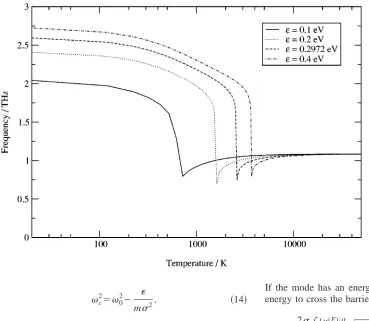
Taken together, the results of Eqs. 共15兲, 共17兲, 共18兲, and 共19兲 allow us to calculate numerically the frequency of an isolated oscillator moving with the mean thermal energy as a function of temperature. Example results are shown in Fig. 1. A typical ‘‘soft-mode’’ behavior is observed, with the fre-quency dropping to zero in a cusp at the transition tempera-ture. This simple approach was used in early studies of MgSiO3.
17
2. Quantum solution
[image:4.612.50.419.55.376.2]The energy eigenfunctions of a particle moving in a sym-metric potential must be either symsym-metric or antisymsym-metric.
FIG. 1. Classical frequency of a double-well oscillator in thermal contact with a heat bath plotted against temperature for various barrier heights ⑀. The other double-well parameters are m⫽1,
0⫽0.0691 eV1/2Å⫺1amu⫺1/2,
and ⫽1.866 amu1/2Å. The fre-quency falls to zero in a cusp at the phase transition. At ⑀
⫽0.2972 eV, the double-well pa-rameters are appropriate for the double-well describing the orthorhombic-tetragonal transition in MgSiO3 at zero pressure共Ref.
Furthermore, by considering building up the Gaussian barrier adiabatically, it is clear that the symmetry of the eigenfunc-tions must be the same as for those of the harmonic oscilla-tor.
The definite symmetry of the wavefunctions leads to a ‘‘paradox’’ for wells of finite separation. If we know the energy of the oscillator then it is in an energy eigenstate and the wave function is either symmetric or antisymmetric. Hence the probability distribution is symmetric about the center of the double well, and we cannot meaningfully say which side the oscillator is confined in, even if its energy is much less than the barrier height. Thus it is not conceptually clear that equating the mean thermal energy with the barrier height gives the correct transition temperature. We discuss this further in Sec. III D.
The Hamiltonian operator for a particle moving in the quadratic potential without the additional Gaussian potential is
Hˆ0⫽⫺ ប
2
2m 2 x2⫹
1
2m0 2
x2. 共20兲
The well-known energy eigenvalues and eigenfunctions for the time-independent Schro¨dinger equation Hˆ0n
⫽En0n are
En0⫽共n⫹1/2兲ប0 共21兲
and
n⫽
2⫺n/2
冑
n!冉
m0ប
冊
1/4e⫺m0x2/2បH n
冉
冑
m0
ប x
冊
共22兲for n苸N0, where Hn(x) is the nth Hermite polynomial.
The Hamiltonian operator for a particle moving in the double well is Hˆ⫽Hˆ0⫹V
1, where V1⫽⑀(e⫺x
2/22
⫺1) is the extra Gaussian term. Let the eigenfunctions and eigenener-gies of the full Hamiltonian ben and En.
The eigenfunctions of the simple harmonic oscillator 共SHO兲are chosen as the basis of wave-function space. This choice makes the computation particularly simple, as will be seen below.
The matrix elements of the Hamiltonian with respect to our chosen basis are
具
i兩Hˆj典⫽具
i兩Hˆ0j典⫹具
i兩V1j典⫽共i⫹1/2兲ប0␦i, j⫹ ⑀
2(i⫹j)/2
冑
i! j !冕
⫺⬁ ⬁e⫺Kz2Hi共z兲Hj共z兲dz,
共23兲
where K⬅ប/2m02⫹1. Note that the matrix is real and symmetric.
The Hermite polynomials satisfy Hi(⫺x)⫽(⫺1)iHi(x),
so that
具
i兩V1j典⫽0 if i⫹j is odd. If i⫹j is even then theintegrand is an even function. Hence, in this case,
具
i兩V1j典⫽2⑀
2(i⫹j)/2
冑
i! j!冕
0 ⬁e⫺Kz2Hi共z兲Hj共z兲dz.
共24兲
The eigenvalues of the matrix of the Hamiltonian are the allowed energy levels. For energies that are large compared with the barrier height the particle will spend most of its time away from the center of the well; hence we expect that the system will behave as a SHO in this limit. Indeed, it is clear from Eq.共24兲that the elements of the matrix
具
i兩V1j典 falloff rapidly as i and j increase. Hence, for large i or j, the eigenstates of the Hamiltonian tend to to those of the SHO. Thus we only need to diagonalize the upper left-hand corner 关say, the (nc⫹1)⫻(nc⫹1) submatrix兴in order to obtain the
first nc⫹1 energy levels E0 to Enc. Beyond nc the
eigen-states may be taken to be those of the SHO. The comparative ease with which the Hamiltonian matrix can be diagonalized is one of the advantages of the quadratic-plus-Gaussian double-well potential over the quartic double-well potential, although there is no analytic form equivalent to Eq.共6兲.
Assuming that nc is sufficiently large, the canonical
par-tition function can be written as
Z⫽
兺
n⫽0
nc
e⫺En⫹
兺
n⫽nc⫹1 ⬁
e⫺(n⫹1/2)ប0
⫽
兺
n⫽0
nc
e⫺En⫹ e
⫺ប0(nc⫹1)
eប0/2⫺e⫺ប0/2
. 共25兲
The free energy of the double-well oscillator can then be evaluated as
F1⫽⫺kBT log共Z兲. 共26兲
C. Practical implementation in the quasiharmonic method
Having proposed that each soft mode at a given wave vector be described by a double well of the form given in Eq. 共9兲, we now describe how the parameters⑀, , and0 can be determined. Note that if 兵xi其 are mass-reduced phonon
coefficients then we may, without loss of generality, set
m⫽1.
Consider the phonon dispersion curve of a crystal struc-ture in which imaginary frequencies are present. Those branches that remain real throughout the whole of the Bril-louin zone are treated as harmonic and, for each mode at each wave vector, Equation共6兲may be used to find the cor-responding free energy. For those branches that are imagi-nary in some region of the Brillouin zone, however, we pro-pose the following treatment.
possible to fit Eq.共9兲to every branch even if the mode is not imaginary since that Eq.共9兲does not necessarily describe a double well. In practice the harmonic approximation is used for all-real branches, it is equivalent to setting⑀⫽0.
共2兲For each branch we use our results for the double-well parameters at the symmetry points to construct interpolating polynomials over the whole of the Brillouin zone for the ⑀ and parameters.
共3兲 For any wave vector in the Brillouin zone, we may find the spectrum of corresponding共possibly imaginary兲 fre-quencies. Provided we know to which branch these modes belong, we have sufficient information to determine the pa-rameters of the appropriate double-well for each mode.⑀and are found by interpolating to our wavevector and the un-stable frequency givesc关see Eq.共14兲兴, from which we may
find 02⫽c2⫹⑀/m2.
共4兲Hence, for any given wave vector, the free energy of each mode, whether harmonic or soft, can be evaluated. These free energies can be summed to give the free-energy contribution from all modes at the given wavevector.
共5兲The free energy can then be integrated over all wave vectors in the Brillouin zone to give the total lattice thermal free energy. By using a grid-based scheme to integrate over an irreducible wedge of the zone and by making use of the continuity of the gradient of each branch, it is possible to keep track of which branch is which—necessary if the ap-propriate values of ⑀ and are to be interpolated in the pressence of imaginary branch crossings. The problem of interpolation over an irreducible wedge of the Brillouin zone has been studied extensively in the context of electronic ei-genvalues: see, for example, Ref. 18.
The high-symmetry dynamically stabilized phase and the low-symmetry ‘‘frozen-phonon’’ phase can now be treated as being distinct. Hence the methodology of Sec. II B can be applied to find the phase diagram.
D. Interpretation of the soft mode transition
Consider an isolated symmetric double-well oscillator. For the probability density to be asymmetric—necessary if we are to meaningfully say that the particle is in one well or the other—we must have a mixture of symmetric and anti-symmetric energy eigenstates. Therefore, we cannot simulta-neously know the energy of our particle and which well it is in unless we break the symmetry共e.g., by allowing the crys-tal to distort under phonon-strain coupling兲.
If the oscillating particle’s wave function is a superposi-tion of different energy eigenfuncsuperposi-tions then the expansion coefficients will evolve in time共provided the system remains both undisturbed and unobserved兲 according to the Schro¨-dinger equation. Hence the quantum mechanical expectation value of the particle’s position
具
x典
changes in time.The time-dependent wave function can be written as
⌿共x,t兲⫽
兺
n⫽0⬁
cne⫺iEnt/បn共x兲. 共27兲
Hence the expectation of x can be written as
具
x典
⫽兺
n⫽0⬁
兺
m⫽0⬁
cn*cmei(En⫺Em)t/ប
具
n兩xm典⫽2
兺
n evenm odd
兺
兩cn兩兩cm兩cos共nmt⫹nm兲
具
n兩xm典,共28兲 where nm⫽兩En⫺Em兩/ប and nm⫽关arg(cm)
⫺arg(cn)兴sgn(nm). Note that we use the fact that
具
n兩xm典⫽0 ifnandmare either both odd or both even,since x itself is odd. We also use the fact that
具
n兩xm典
⫽
具
m兩xn典.We assume that the energy levels are initially populated according to Boltzmann statistics; thus 兩cn兩2⫽Z⫺1e⫺En,
where ⫽1/kBT and Z⫽兺⬁n⫽0e⫺En is the canonical
parti-tion funcparti-tion. So we have
具
x典
⫽兺
n evenm odd
兺
⌫nmcos共nmt⫹nm兲, 共29兲
where⌫nm⫽2Z⫺1e⫺(En⫹Em)/2
具
n兩xm典 is the amplitude ofthe sinusoidal component in the expansion of
具
x典
with fre-quency nm.For the harmonic-oscillator potential, the frequencies of the oscillations in
具
x典
are of the form nm⫽兩En⫺Em兩/ប⫽兩n⫺m兩0. Thus the lowest oscillation frequency is 0. For the symmetric double well, however, we end up with a set of pairs of energy levels that are very close to each other 共becoming degenerate in the limit that the barrier height goes to infinity兲. These give rise to oscillation frequencies very much lower than 0.
As the temperature is increased, higher-frequency compo-nents have larger ⌫ coefficients. We suggest that the soft-mode phase transition be judged to occur when the frequency with the highest coefficient exceeds the frequency of the ex-perimental probe. When this has happened, the predominant sinusoidal component of
具
x典
has a frequency higher than can be measured by the experimental probe, and so it appears to the experimenter that具
x典
⫽0. Below this temperature, mea-surements of具
x典
will tend to find it in one well or the other. This definition is different from the polymorphic one 共Sec. II B兲because of the contribution to the free energy from the symmetry-breaking distortion of the lattice that inevitably accompanies the transition. In particular, the quasiharmonic transition is first-order while this measurement dependent ‘‘soft-mode’’ one is second order.16Thus the first-order transition is determined by comparing 共1兲 the free energy of the soft-mode phase, calculated as above, expanded about an unstable frozen-ion structure with-out strain-phonon coupling, with 共2兲 the free energy of the low symmetry phase, calculated by expanding about the minimum of total energy. Typically, the former will have a higher entropy 共sampling from both wells兲, while the latter has a lower energy.
E. Absorption of low-frequency photons
the two energies (En⫹En⫺1)/2 for the quantum double-well oscillator. Absorption of photons at frequency (En
⫺En⫺1)/ប is symmetry allowed.
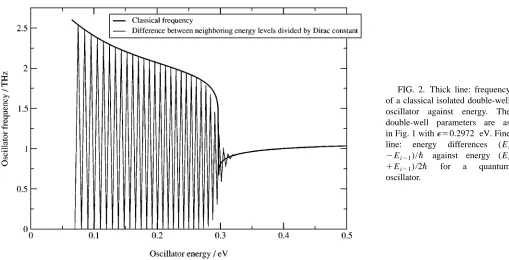
For energies in excess of the barrier height the frequency (En⫺En⫺1)/ប is virtually identical to the classical fre-quency for energy (En⫹En⫺1)/2, obtained using the method of Sec. III B 1. In the very high-energy limit the frequency behaves as that of the quadratic potential well without the Gaussian barrier.
For energies less than the barrier height the energy levels tend to degenerate pairs of levels. The frequencies given by the difference between the energy levels of neighboring pairs again correspond to the classical frequencies. However, the pairs of almost-degenerate eigenstates imply the existence of very low-frequency absorption peaks. 共These are the very low frequencies that alternate with the classical frequencies below the transition energy in Fig. 2.兲It should be noted that these frequencies are not associated with the normal modes of the low-symmetry phase and do not, therefore, contribute to the quasiharmonic thermal energy. They are a feature of the quantum double-well oscillator without a classical analog.
IV. APPLICATION OF QUASIHARMONIC METHODS TO PERICLASE
A. Computational details
1. Cold curve
For each lattice parameter the total energy is evaluated using theCASTEPsoftware package,19which utilizes density-functional theory in the generalized gradient approximation 共GGA兲.20 The ionic cores are accounted for using ultrasoft pseudopotentials21 in Kleinman-Bylander form.22 The wave functions of the valence electrons are expanded in a plane-wave basis set up to an energy cutoff of 540 eV.
For the B1 phase, the simulation cell consists of a single cubic unit cell. The Brillouin zone is sampled at 20 special points generated from an 8⫻8⫻8 mesh using the Monkhorst-Pack scheme.23For the B2 phase, the simulation cell is a single cubic primitive cell. The Brillouin zone is sampled at 35 special points from a 9⫻9⫻9 mesh. In each case the point symmetries of the crystal are enforced.24
The equilibrium lattice parameter of the B1 phase at zero external pressure共which corresponds to the minimum of the cold-curve兲 calculated using CASTEP is a⫽4.259 Å, which may be compared with an experimentally determined param-eter a⫽4.2115(1) Å.28The difference between the theoret-ical and experimental values is about 1%.
2. Determination of the matrix of force constants
The supercells simulated to determine the matrices of force constants for the B1 phase consist of 2⫻2⫻2 cubic unit cells共64 atoms兲. Thus the interactions between a given ion and its third-closest shell of neighbors are included in our calculations. For the B2 phase, the cells used consist of 2
⫻2⫻2 cubic primitive unit cells共16 atoms兲. In these super-cells the crystal symmetry is such that only two ionic dis-placements are required to complete the entire matrix of force constants. The plane-wave cutoff energy is 540 eV and the Brillouin zone is sampled at six special points from a 4
⫻4⫻4 mesh. In each simulation the ion displaced from equilibrium is moved by 0.4% of the lattice parameter.
[image:7.612.50.559.51.311.2]As demonstrated by Parlinski et al.,12it is possible to cal-culate the Born effective charge tensors from first principles using simulations of elongated supercells. Note that because of the symmetry of the B1 and B2 phases, the Born effective charge tensors are isotropic 共so Zn,␣,⫽Zn␦␣,). Further-more, the sum of the Born effective charges over the ions in a unit cell must be zero14 共so ZMg⫽⫺ZO). Hence there is
FIG. 2. Thick line: frequency of a classical isolated double-well oscillator against energy. The double-well parameters are as in Fig. 1 with⑀⫽0.2972 eV. Fine line: energy differences (Ei ⫺Ei⫺1)/ប against energy (Ei ⫹Ei⫺1)/2ប for a quantum
effectively only one undetermined parameter in the nonana-lytic term: ZMg(0)/
冑
⑀0(0).We choose ZMg(0)/
冑
⑀0(0)⫽4.4 to give the LO branch in the dispersion curve of Fig. 3. Our values for the effective charge tensors of the B1 phase are such that the calculated LO branch for lattice parameter 4.2 Å are in reasonable agreement the experimental results of Peckham.25We neglect the variation of the effective charge tensors with lattice pa-rameter.B. Approximations and errors
1. Errors in ab initio total-energy calculations
Total-energy differences between structures calculated us-ing density-functional theory in the generalized gradient ap-proximation are thought to be reliable to within a few percent.22 The cutoff energy of the plane-wave basis at 540 eV is sufficient for convergence of the total energies of the crystals to within 10 eV per ion, several orders of magnitude less than the likely error due to the use of the GGA. The Hellmann-Feynman forces are converged to within 1 meV Å⫺1, at least two orders of magnitude less than the dominant forces arising when an ion is displaced.
2. Harmonic approximation
We investigate the range of validity of the harmonic ap-proximation. This is done for the B1 phase with a lattice parameter a⫽4.2 Å.
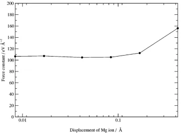
We evaluate the force constant of the restoring force on a magnesium ion as it is displaced in the x direction. The re-sults are shown in Fig. 4. It can be seen that the force con-stant starts to increase when the ionic displacement reaches
amax⬇0.084 Å, about 2% of the lattice parameter, at which point the potential energy is about 0.4 eV. Other
displace-ments are similar; hence it is reasonable to assume that the forces remain linear 共and the quasiharmonic assumption is valid兲for temperatures up to several thousand K.
3. Other sources of error
Another potential source of error is the limited size of the simulation supercells. However, the results shown in Table I for the B1 phase make it clear that interactions beyond the third-closest shell of neighbors may be safely neglected.26 Contributions to the free energy from the thermal excitation of the valence electrons, from coupled electron-phonon ex-citations and from the equilibrium population of defects are thought to be negligible in comparison with the frozen-ion and lattice thermal energies.15
A poor convergence of the Hellmann-Feynman forces can result in the violation of Newton’s third law for the matrix of force constants. Typically this results in the acoustic branches of the dispersion curve failing to pass through zero at the center of the Brillouin zone.11 As discussed in Sec. II A 2, Newton’s third law is imposed on the matrix of force constants. However, even without this, the calculated acous-tic branches pass very close to zero at the zone center.
The method by which long-range polarization effects are accounted for is also approximate. The effects of this are discussed below.
C. Ab initio phonons
1. B1 phase
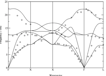
Inelastic neutron-scattering experiments were carried out by Peckham,25and used to generate dispersion curves for the
B1 phase.27 We compare our theoretical dispersion curve with these results in Fig. 3. 共Note that our dispersion curve was generated for a lattice parameter of 4.2 Å, whereas
Peck-FIG. 3. Dispersion curves for
B1 MgO at a lattice parameter 4.2
Å. The symmetry points in the dispersion curve are共from left to right兲 ⌫ 关000兴, X关001兴, X关011兴,⌫
关000兴, and L 关12 1 2 1
2兴. Note the
LO-TO splitting共at⌫, the LO fre-quency is 22.0 THz whereas the TO frequency is 12.4 THz兲arising from the nonanalytic term of Eq.
[image:8.612.53.418.56.319.2]ham’s results were obtained under ambient conditions where the lattice parameter is 4.212 Å.兲Our theoretical results are in reasonable agreement with experiment. 共The lattice pa-rameter of 4.2 Å corresponds to a pressure of about 7 GPa at zero temperature.兲
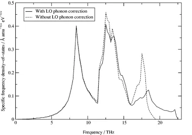
The specific frequency density-of-states function is shown in Fig. 5. Without the addition of the nonanalytic term to the dynamical matrix, the longitudinal optic branch is degenerate with the transverse optic branch at the ⌫ point, and this is also shown. Although only the LO branch is altered substan-tially, it can be seen that the inclusion of the nonanalytic term has a significant effect on the density of states.
We compare sound velocities calculated from our disper-sion curves with the experimental results of Reichmann
et al.28 obtained using ultrasonic interferometry. Reichmann
et al. obtained a P-wave sound speed of 9119 ms⫺1 in the 关100兴 direction, whereas our longitudinal-acoustic mode has (dLA/dk[100])k⫽0⫽11367 ms⫺1. On the other hand, in the 关111兴 direction, the experimental P-wave velocity is 10125 ms⫺1, which may be compared with our theoretical value of 10818 ms⫺1.
Thus Reichmann et al.’s experimental results show a higher degree of anisotropy than do our theoretical results. The discrepancy would appear to be共at least partly兲caused by the imposition of symmetry and Newton’s third law on the matrix of force constants:11 if this procedure is not carried out then we find that (dLA/dk[100])k⫽0
⫽10770 ms⫺1 and (dLA/dk
[111])k⫽0⫽12651 ms⫺1. Al-though Reichmann et al.’s P-wave velocities are still some-what less than these theoretical velocities, both are now in agreement that the velocity in the关100兴direction is less than the velocity in the 关111兴 direction.
2. B2 phase
Typical dispersion curves for the B2 phase at lattice pa-rameters 2.0 and 2.7 Å are shown in Figs. 6 and 7. At zero temperature these lattice parameters correspond to pressures of 653 GPa and ⫺6 GPa, respectively.
Note the presence of unstable modes at low pressures in the dispersion curve of the B2 phase 共Fig. 7兲. We find that the B2 phase is structurally unstable for pressures below about 82 GPa. In our calculations for the phase boundary in periclase we do not require our method for dealing with soft modes, because the imaginary frequencies are only found in the B2 phase at pressures for which the B1 phase is clearly favored.
D. Ab initio equation of state
[image:9.612.52.420.55.323.2]We plot the pressure against specific volume for a range of temperatures in Fig. 8. This is the desired thermodynamic equation of state for periclase. Also shown is a third-order Birch-Murnaghan equation of state generated from the iso-thermal bulk modulus and its first derivative with respect to volume, which were obtained by means of ultrasonic sound velocity measurement.29
TABLE I. Magnitude of the component of force in the 关001兴 direction when the Mg ion at共0,0,0兲is displaced in the关001兴 direc-tion by 0.05% of the length of a 1/
冑
2⫻1/冑
2⫻8 supercell. Coordi-nates are given as fractions of the supercell dimensions. 共These results are for B1 MgO at a lattice parameter 4.2 Å.兲Magnitude of关001兴component
Position of Mg atom of force / eV Å⫺1
共0,0,0兲 0.13424
共0.5,0.5,0.0625兲 0.03356
共0,0,0.125兲 0.00981
[image:9.612.52.297.647.734.2]共0.5,0.5,0.1875兲 0.00006
FIG. 4. Graph of the restoring force divided by the finite dis-placement of a Mg ion in the
As a test of the validity of our results, the isothermal bulk modulus at zero temperature and external pressure 共where periclase is entirely in the B1 phase兲can be compared with experimental results. We calculate the bulk modulus to be
⫺v(p/v)T,v⫽155 GPa, whereas an experimentally deter-mined value is 160.3⫾0.3 GPa.29 The theoretical and ex-perimental results differ by about 3%.
We may also compare the pressure derivative of the bulk modulus at zero pressure and temperature with experimental results. The bulk modulus is found to be almost, but not quite, a linear function of pressure. Fitting a straight line to
the data from⫺8.3 to 21.12 GPa we find that the the gradi-ent is 4.11, in excellgradi-ent agreemgradi-ent with the experimgradi-entally determined value of 4.2⫾0.2.29It is found that the pressure derivative of the bulk modulus decreases slightly as the pres-sure is increased.
E. Ab initio phase diagram
The theoretical phase diagram of solid periclase is shown in Fig. 9. At pressures and temperatures below and to the left of the phase boundary shown in the diagram, periclase exists in the B1 phase; above and to the right of the boundary it
[image:10.612.53.432.56.322.2]FIG. 5. Specific frequency density of states for the B1 phase at a lattice parameter 4.2 Å with and without the inclusion of the nonanalytic term in the dynamical matrix.
FIG. 6. Dispersion curves for
B2 MgO at a lattice parameter 2.0
Å. The symmetry points in the dispersion curve are共from left to right兲 X 关1200兴, ⌫ 关000兴, M 关1
2 1 20兴, R关
1 2 1 2 1
2兴, ⌫ 关000兴, and X 关1
[image:10.612.51.418.476.728.2]exists in the B2 phase. Duffy et al.30showed experimentally that, at room temperature, the B1 phase is stable to pressures of at least 227 GPa. This lies well within the B1 region of our theoretical phase diagram. It can also be noted that the
B2 phase is not favored at the pressures at which it is
struc-turally unstable.
Also shown in Fig. 9 is the theoretical phase diagram obtained by Strachan et al.31 using a molecular-dynamics simulation. Although qualitatively similar, the calculated po-sition and orientation of the B1-B2 phase boundary is very
different. Karki et al.5 obtained a B1-B2 transition pressure of 460 GPa at 0 K, which also differs substantially from that of Strachan et al. Figure 10 shows the Gibbs free energy plotted against pressure for the two phases at two different temperatures. The difficulty in ascertaining the transition pressures at which the curves cross is apparent. This consid-eration will affect all theoretical calculations of the phase diagram of periclase.
[image:11.612.51.424.56.318.2]We confirm the difficulty in locating the transition by at-tempting to reproduce Karki et al.’s zero-temperature results,
FIG. 7. Dispersion curves for
B2 MgO at a lattice constant of
2.7 Å. The symmetry points are as in Fig. 6. Note the branches of imaginary phonon frequencies, in-dicating that the structure is me-chanically unstable at this volume.
[image:11.612.49.420.466.725.2]in which zero-point lattice vibrational energy is neglected. We simply calculate the enthalpy against pressure for the two phases using CASTEP. The results are shown in Fig. 11. We find a transition pressure of 664 GPa, different from that of Karki et al. 共460 GPa兲. The possibility of a metallization transition lowering the energy of the B2 phase was investi-gated but found not to occur at relevant pressures.
We consider the fractional error in unit-cell volume for the B2 phase to which the difference between the specific enthalpies of the B1 and B2 phases at 451 GPa corresponds.
For a given unit-cell enthalpy for the B2 phase, we find the fractional volume difference as
冏
⌬V V冏
⫽2冏
hB2⫺hB1
hB2⫹hB1
冏
, 共30兲
where hB1⫽⫺34.4043 eV Å⫺3 and hB2⫽⫺34.3978
eV Å⫺3 are the specific enthalpies of the two phases at 451 GPa. Thus a discrepancy of ⌬V/V⫻10⫺4⬇0.02% in the volume of either phase would correspond to a 200-GPa
FIG. 9. Theoretical phase dia-gram of periclase. The B1 phase region is below and to the left of the B1-B2 coexistence line. Also shown are other theoretical results
共Refs. 5 and 31兲, including a the-oretical B1-liquid phase bound-ary.
change in the transition pressure. This illustrates the sensi-tivity of the transition point to the details of how the total-energy calculations are carried out.
We use the generalized gradient approximation and ultra-soft pseudopotentials,20,21 whereas Karki et al. used the local-density approximation and Qc-tuned
pseudopo-tentials.32,33The difference between calculated volume using these two methods is typically of the order of 5%; hence this is likely to be responsible for the difference between our results and Karki et al.’s.
The Clausius-Clapeyron equation for the coexistence line between two phases in ( p,T) space is
d p
dT⫽
⌬s
⌬v, 共31兲
where p(T) is the coexistence line and ⌬s and ⌬v are the specific entropy and volume differences between the two phases across the line. At zero temperature the entropy of the two phases should be zero by the third law of thermodynam-ics which is valid within our method 共though not, e.g. in classical molecular dynamics31兲; therefore, provided the phases have different densities, the coexistence line should satisfy d p/dT⫽0 at T⫽0. Fig. 9兲does not appear to satisfy this requirement.
The explanation for this apparent discrepancy lies with the fact that the densities of the two phases are very similar 共and converging兲 at their predicted zero-temperature transi-tion point: the specific volumes of the B1 and B2 phases are 0.202 and 0.198 Å3amu⫺1, respectively.
V. CONCLUSIONS
We have described an extension to the quasiharmonic method that allows the free-energy contribution from ‘‘soft’’ phonons in dynamically stabilized crystals to be evaluated.
Our approach is based on a form of potential double-well different for that used in previous work on soft phonons: a parabola-plus-Gaussian form that has the advantage of being harmonic in both the low- and high-temperature limits.
We argue that the first-order nature of the phase transi-tions found using our extended quasiharmonic method arises because of the coupling of the relevant phonon to strain in the crystal. Without this coupling, the transition would be second order. We have suggested a criterion for judging when a second-order soft-mode phase transition has oc-curred, taking into account the quantum-mechanical nature of the problem.
At energies less than the height of the central barrier in our symmetric potential double well, the allowed energy lev-els consist of near-degenerate pairs. Hence we suggest there must exist extremely low-frequency photon absorption peaks for soft-mode materials in their low-temperature phase, cor-responding to photon-induced transitions between such pairs. We have evaluated the equation of state and the phase boundary for the B1-B2 transition in periclase using ab
ini-tio calculaini-tions in the quasiharmonic approximaini-tion. We
pre-dict that this transition will occur, but that it is well outside the ranges encountered inside the Earth. Locating the B1-B2 phase boundary with precision is difficult, however, because the Gibbs free energy curves of the two phases are very similar when they cross.
ACKNOWLEDGMENTS
[image:13.612.54.370.55.316.2]We would like to thank D. C. Swift and M. C. Warren for helpful discussion. This work was carried out as part of the UKCP-MSI collaboration, supported by EPRSC GR/ N02337. Copies of the codes used for the free-energy calcu-lations are available from the authors on request.
FIG. 11. Enthalpy h⫽e⫹pv
plotted against pressure for the B1 and B2 phases of MgO at a tem-perature 0 K共note that zero-point energy is not included in the re-sults shown on this graph兲. The curves cross 共and so the phase transition is predicted to occur兲at 664 GPa. These results are ob-tained directly from the results of
1D. C. Wallace, Thermodynamics of Crystals共Wiley, New York,
1972兲.
2M. Born and K. Huang, Dynamical Theory of Crystal Lattices
共Oxford University Press, London, 1956兲.
3W. Zhong, D. Vanderbilt, and K.M. Rabe, Phys. Rev. B 52, 6301
共1995兲.
4M.C. Warren, G.J. Ackland, B.B. Karki, and S.J. Clark, Miner.
Mag. 62, 585共1998兲.
5B.B. Karki, G.J. Ackland, and J. Crain, J. Phys.: Condens. Matter
9, 8579共1997兲.
6M.C. Warren and G.J. Ackland, Phys. Chem. Miner. 23,共1996兲. 7M. C. Warren, Ph.D. thesis, The University of Edinburgh, 1997. 8G. Fiquet, A. Dewaele, D. Andrault, M. Kunz, and T. Le Bihan,
Geophys. Res. Lett. 27, 21共2000兲.
9K. Parlinski and Y. Kawazoe, Eur. Phys. J. B 16, 49共2000兲. 10A.R. Oganov, J.P. Brodholt, and G.D. Price, Phys. Earth Planet.
Inter. 122, 277共2000兲.
11
G.J. Ackland, M.C. Warren, and S.J. Clark, J. Phys.: Condens. Matter 9, 7861共1997兲.
12K. Parlinski, J. Łaz˙ewski, and Y. Kawazoe, J. Phys. Chem. Solids
61, 87共2000兲.
13N. W. Ashcroft and N. D. Mermin, Solid State Physics共Saunders
College Publishing, Philadelphia, 1976兲.
14W. Cochran and R.A. Cowley, J. Phys. Chem. Solids 23, 447
共1962兲.
15D. C. Swift and G. J. Ackland, Phys. Rev. B 64, 214107共2001兲;
D. C. Swift, Ph.D. thesis, The University of Edinburgh, 2000.
16A.D. Bruce, Adv. Phys. 29, 117共1980兲.
17L. Stixrude and R.E. Cohen, Nature共London兲364, 613共1993兲. 18P.E. Blo¨chl, O. Jepsen, and O.K. Andersen, Phys. Rev. B 49,
16 223共1994兲.
19CASTEP 3.9, academic version, licensed under the UKCP-MSI
Agreement www.cse.clrc.ac.uk/Activity/UKCP共1999兲.
20J.P. Perdew, J.A. Chevary, S.H. Vosko, K.A. Jackson, M.R.
Ped-erson, D.J. Singh, and C. Fiolhais, Phys. Rev. B 46, 6671
共1992兲.
21D. Vanderbilt, Phys. Rev. B 41, 7892共1990兲.
22M.C. Payne, M.P. Teter, D.C. Allan, T.A. Arias, and J.D.
Joan-nopoulos, Rev. Mod. Phys. 64, 1045共1992兲.
23H.J. Monkhorst and J.D. Pack, Phys. Rev. B 16, 2981共1977兲. 24K. Kunc, R. J. Needs, O. J. Nielsen, and R. M. Martin共
unpub-lished兲.
25G. Peckham, Proc. Phys. Soc. London 90, 654共1967兲.
26Apart from the nonanalytic dipole term, which is calculated
sepa-rately.
27M.J.L. Sangster, G. Peckham, and D.H. Saunderson, J. Phys. C 3,
1026共1970兲.
28H.J. Reichmann, S.D. Jacobsen, S.J. Mackwell, and C.A.
McCammon, Geophys. Res. Lett. 27, 799共2000兲.
29
I. Jackson and H. Niesler, in High Pressure Research in
Geophys-ics, edited by S. Akimoto and M.H. Manghnani共Center for Aca-demic Publication, Tokyo, 1982兲, pp. 93–113.
30T.S. Duffy, R.J. Hemley, and H.-K. Mao, Phys. Rev. Lett. 74,
1371共1995兲.
31A. Strachan, T. C¸ ag˘in, and W.A. Goddard, Phys. Rev. B 60,
15 084共1999兲.
32J.P. Perdew and A. Zunger, Phys. Rev. B 23, 5048共1981兲. 33J.S. Lin, A. Qteish, M.C. Payne, and V. Heine, Phys. Rev. B 47,
4174共1993兲; M. H. Lee Ph.D. Thesis, University of Cambridge, UK, 1995.
34In fact, if we have calculated the total energy of the