Evolution and characteristics of global pc5 ULF waves during a high solar wind speed interval

Evolution and characteristics of global Pc5 ULF waves during a high

solar wind speed interval

I. J. Rae,1 E. F. Donovan,2 I. R. Mann,1 F. R. Fenrich,1C. E. J. Watt,1D. K. Milling,1 M. Lester,3 B. Lavraud,4J. A. Wild,3,5 H. J. Singer,6 H. Re`me,7 and A. Balogh8

Received 5 January 2005; revised 16 August 2005; accepted 12 September 2005; published 15 December 2005.

[1] We present an interval of extremely long-lasting narrow-band Pc5 pulsations during the

recovery phase of a large geomagnetic storm. These pulsations occurred continuously for many hours and were observed throughout the magnetosphere and in the dusk-sector ionosphere. The subject of this paper is the favorable radial alignment of the Cluster, Polar, and geosynchronous satellites in the dusk sector during a 3-hour subset of this interval that allows extensive analysis of the global nature of the pulsations and the tracing of their energy transfer from the solar wind to the ground. Virtually monochromatic large-amplitude pulsations were observed by the CANOPUS magnetometer chain at dusk for several hours, during which the Cluster spacecraft constellation traversed the dusk magnetopause. The solar wind conditions were very steady, the solar wind speed was fast, and time series analysis of the solar wind dynamic pressure shows no significant power concentrated in the Pc5 band. The pulsations are observed in both geosynchronous electron and magnetic field data over a wide range of local times while Cluster is in the vicinity of the magnetopause providing clear evidence of boundary oscillations with the same periodicity as the ground and geosynchronous pulsations. Furthermore, the Polar spacecraft crossed the equatorial dusk magnetosphere outside of geosynchronous orbit (L6 –9) and observed significant electric and magnetic perturbations around the same quasi-stable central frequency (1.4 –1.6 mHz). The Poynting vector observed by the Polar spacecraft associated with these pulsations has strong field-aligned oscillations, as expected for standing Alfve´n waves, as well as a nonzero azimuthal component, indicating a downtail component to the energy propagation. In the ionosphere, ground-based magnetometers observed signatures characteristic of a field-line resonance, and HF radars observed flows as a direct

consequence of the energy input. We conclude that the most likely explanations is that magnetopause oscillations couple energy to field lines close to the location of Polar, setting up standing Alfve´n waves along the resonant field lines which are then also observed in the ionosphere. In the absence of monochromatic dynamic pressure variations in the solar wind, this event is a potential example where discrete frequency pulsations in the magnetosphere result from the excitation of a magnetospheric waveguide mode, perhaps excited via the Kelvin-Helmoltz instability or via overreflection at the duskside

magnetopause.

Citation: Rae, I. J., et al. (2005), Evolution and characteristics of global Pc5 ULF waves during a high solar wind speed interval, J. Geophys. Res.,110, A12211, doi:10.1029/2005JA011007.

1. Introduction

[2] Global ultra low frequency (ULF) oscillations in the

Earth’s magnetosphere are believed to play a significant role in the mass, energy, and momentum transport within the Earth’s magnetosphere. For example, ULF waves accelerate auroral electrons [e.g.,Lotko et al., 1998] and are thought to play a role in mass transport [e.g.,Allan et al., 1990] and the energization and transport of radiation belt electrons [e.g., Elkington et al., 1999]. Standing mode ULF oscillations on magnetospheric field lines were first postulated byDungey [1955]. These ULF perturbations can be excited externally (i.e., by the solar wind) or internally (via resonance with energetic particle sources [e.g. Southwood et al., 1969]). 1_{Department of Physics, University of Alberta, Edmonton, Alberta,}

Canada.

2

Department of Physics and Astronomy, University of Calgary, Calgary, Alberta, Canada.

3

Department of Physics and Astronomy, University of Leicester, Leicester, UK.

4

Los Alamos National Laboratory, Los Alamos, New Mexico, USA.

5_{Also at Department of Communication Systems, Lancaster University,}

Lancaster, UK.

6_{NOAA Space Environment Center, Boulder, Colorado, USA.} 7

Centre d’Etude Spatiale des Rayonnements, Tolouse, France.

8

Physics Department, Imperial College London, London, UK.

External solar wind drivers of ULF waves in the magne-tosphere include the Kelvin-Helmholtz Instability (KHI) via surface waves [e.g., Southwood, 1974; Chen and Hasegawa, 1974], direct solar wind ram pressure changes [e.g.,Kepko et al., 2002], solar wind discontinuities [Allan et al., 1986; Wright, 1994], solar wind buffeting [Wright and Rickard, 1995], sudden impulses [Mathie and Mann, 2000], or wave overreflection [Mann et al., 1999].

[3] ULF cavity modes [e.g., Kivelson et al., 1984;

Kivelson and Southwood, 1985] were first postulated to support the observations of nearly monochromatic ULF wave activity over a range of Lshells. In this scenario the magnetosphere could act as a resonant cavity when solar wind impulse events or density perturbations impact on the near-Earth environment. Further studies [e.g.,Walker et al., 1992; Samson et al., 1992a, 1992b] developed the wave-guide model, whereby the magnetosphere is open downtail and allows fast mode wave energy to propagate antisunward down the magnetospheric waveguide. In the open wave-guide model, narrow-band compressional waves excited by a broadband source in the solar wind are confined between the magnetopause and an internal turning point in the magnetosphere. The resonant frequencies that are produced by these bounded standing waves are discrete and, if both boundaries are highly reflective, long-lasting. Mann et al. [1999] extended this theory and presented a model for the excitation of magnetospheric waveguide modes during fast solar wind speed intervals by overreflection at the magne-topause. The compressional cavity waveguide modes may excite field line resonances (FLRs) where the frequency of the compressional waves matches the local standing mode FLRs field line eigenfrequency.

[4] There has been extensive evidence presented in the

literature that KHIs at the magnetopause can drive broad-band ULF wave energy into the magnetosphere. Miura [1987] presented simulations of magnetopause KHI-driven ULF wave activity in the magnetosphere in the 3 – 10 mHz range. Further work byAnderson et al.[1990] andLessard et al. [1999a] showed observationally that the same broad frequency range of ULF wave power may be observed in the magnetosphere, the frequency of which was highly dependent on Lshell. However, there are few examples of narrow-band oscillations driving discrete frequency FLRs. Lessard et al. [1999b] presented both ground- and space-based observations of a discrete frequency FLR most likely driven by a solar wind impulse excited waveguide mode. Furthermore, Mann et al. [2002] presented observations from a high solar wind speed interval where the Cluster spacecraft constellation crossed the dusk-sector magneto-sphere and observed what were identified to be K-H driven magnetopause oscillations, in conjunction with quasi-stable global magnetospheric oscillations seen in the ionosphere. Their paper was the first observation-based study suggest-ing a connection between a quasi-stable central frequency of magnetopause oscillations and narrow-band ionospheric ULF cavity/waveguide mode activity. In their paper,Mann et al.[2002] presented comprehensive ground-based obser-vations of FLR characteristics using magnetometer, high-frequency (HF) radar, and optical data. The principal result was the demonstration that KHI on the magnetopause likely produced discrete frequency global ULF wave activity during periods of high solar wind speed, perhaps by a

discrete frequency magnetospheric waveguide mode which is energized by the overreflection mechanism discussed by Mann et al.[1999].

[5] The subject of how an external driving mechanism

can produce FLRs deep inside the magnetosphere is a topic of much debate.Walker[1981] considered the properties of K-H surface waves on the magnetopause and found that if the wavelength on the magnetopause is of the order of ten times the thickness of the boundary, d (kyd0.5 – 0.8), then

there is a preferred and finite wavelength which the growth rate is a maximum and Pc3 – Pc5 perturbations can be excited. These modes hence have quite large azimuthal wave numbers, m or ky.

[6] One alternative way to drive discrete frequency

per-turbations with these frequencies but with smaller m is cavity/waveguide theory [e.g., Mann et al., 1999; Mills et al., 1999]. Waveguide theory has two advantages over the simple evanescent surface mode. First, the amplitude of the excited ULF wave energy does not generally decay spatially away from the magnetopause; rather, the modes propagate radially into the magnetosphere. Second, waveguide theory predicts that the magnetosphere can act as a cavity which traps discrete frequency compressional mode energy. In this scenario a structured spectrum of discrete harmonic fre-quencies should be observed which are determined by the size of the magnetospheric cavity. For waveguide modes which are energized by shear flow at the magnetopause [e.g., Mann et al., 1999] the growth rate of the discrete frequency modes can have maxima at finite and low-m [e.g., Mann et al., 1999, Figure 7]. In this way, discrete frequency waveguide modes, energized by large magneto-sheath shear flows, can drive FLRs deep inside the magnetosphere.

[7] In this paper we consider global ULF pulsations in

a study similar to Mann et al. [2002]. The interval presented concerns a subsection of a period of fast solar wind speed (<850 kms 1) event from 24 to 26 November 2001. A remarkable array of instrumentation was avail-able during this interval, and we concentrate on several hours on 25 November 2001 when the Cluster constella-tion was traversing the dusk sector magnetopause and when Polar was also in a favorable location. The energy deposited into the magnetosphere via magnetopause boundary oscillations is followed through the magneto-sphere into an FLR and down into the Earth’s ionomagneto-sphere. The satellite observations in situ are supplemented by ground-based mesoscale measurements of the magnetic fluctuations as well as the ionospheric flows monitored by high-frequency (HF) radars.

2. Instrumentation

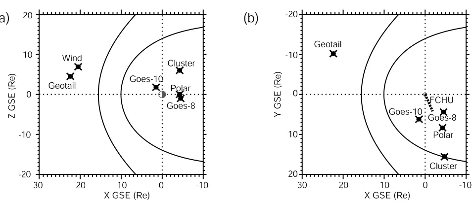
[8] Figure 1 shows the positions of the relevant spacecraft

1998] spacecraft was situated at [X GSE, Y GSE, Z GSE]

[230, 40, 10]REat 0200 UT and for clarity is not included in Figure 1; similarly, the Wind spacecraft [Acuna et al., 1995] was situated at [XGSE, YGSE, ZGSE][20, 77, 7]

REand is not included in Figure 1b for clarity. There were three available solar wind monitors in differing positions in the solar wind (ACE, Wind, and Geotail) and a number of spacecraft were situated in the duskside magnetosphere. The Cluster spacecraft were outbound across the dusk magnetopause, Polar was traversing the duskside magneto-sphere situated close to the equator, and the geosynchro-nous GOES-8, -9, -10, and -12 spacecraft were also all on the dusk flank. GOES-9 and -12 are not shown in Figure 1 for clarity but are around geosynchronous orbit and be-tween GOES-8 and -10. Similarly, for clarity the LANL spacecraft are not shown in Figure 1. Figure 2 shows the ionospheric footprints of these spacecraft and the ground instrumentation used in this study in magnetic local time (MLT): magnetic latitude (MLAT) in AACGM coordinates [Baker and Wing, 1989] with noon at the top of the page, looking down on the northern hemisphere ionosphere at 0200 UT on 25 November 2001. The satellite trajectories were mapped into the ionosphere using the Tsyganenko 89c [Tsyganenko, 1989] magnetic field model (withKp= 2).

[9] In this paper we monitor the solar wind conditions

using data from the magnetometer (MAG) [Smith et al., 1998] and the solar wind proton alpha monitor (SWEPAM) [McComas et al., 1998] on the ACE spacecraft and the Magnetic Fields Instrument (MFI) [Lepping et al., 1995] and Solar Wind Experiment (SWE) [Ogilvie et al., 1995] on the Wind spacecraft. In situ data for the magnetosphere is obtained from the Magnetic Fields Experiment (MFE) [Russell et al., 1995] and Electric Fields Instrument (EFI) [Harvey et al., 1995] on Polar; the Los Alamos National Laboratory (LANL) Synchronous Orbit Particle Analyzer (SOPA) [Belian et al., 1992]; the GOES [Singer et al.,

1996] and Cluster Fluxgate (FGM) [Balogh et al., 1997] Magnetometers; and Cluster Ion Spectrometer instruments [Re`me et al., 2001] (the ion data from the Hot Ion Analyzer (HIA)). To complement the extensive space-based instru-mention, we use ground-based data from the CANOPUS [Rostoker et al., 1995] and SAMNET [Yeoman et al., 1990] magnetometer networks and the SuperDARN HF radar system [Greenwald et al., 1995].

3. Observations on 25 November 2001

3.1. Interplanetary Conditions

[10] Data from the ACE (black) and Wind (grey)

space-craft are shown in Figure 3 for the 25 November 2001, 0100 – 0400 UT. The data have not been lagged; the IMF phase fronts appear to be highly tilted (i.e., negligible IMF By compared to large and positive Bxand Bz) and hence

impinge on each spacecraft almost concurrently. A time delay of 34 min is calculated between the spacecraft and the magnetopause via the method ofKhan and Cowley[1999], though this lag is not added to the figure. Geotail was situated close to the Earth and observed similar solar wind features; Geotail data is not added to the figure for clarity. During the interval the IMF Bx component was large and

positive and initially had a maximum amplitude of14 nT decreasing until0400 UT when Bxapproached zero. The

IMF Bycomponent fluctuated between 3 < By< +6 nT

during the interval, and the IMF Bz component was large

and positive and varied between10 and 16 nT. The solar wind velocity remained approximately constant between 750 and 800 km s 1until 0245 UT, when it dropped to 650 – 700 km s 1. The dynamic pressure, Psw, fluctuated but

remained around1.5 – 2 nPa. An FFT analysis of the time-shifted ACE, Wind, and Geotail (not shown) dynamic pressure data between 0100 and 0400 UT revealed no significant peaks that might be responsible for directly

exciting monochromatic magnetospheric waves by the mechanism proposed by Kepko et al.[2002].

3.2. Dusk-Sector Magnetopause Measurements

[11] The Cluster spacecraft were outbound through the

magnetopause in the dusk sector in the early UT hours on 25 November 2001. The FGM instruments on all four spacecraft switched on at around 0100 UT. From top to bottom, Figure 4a shows data from 0200 to 0300 UT of the CIS HIA ion spectra and derived ion velocity magnitudes from Cluster 1, together with total magnetic field (Btotal)

from all four spacecraft. Figure 4b shows normalized power spectral analysis of (top) Btotal from Cluster 1 – 4 and

(bottom) CIS ion velocities from Cluster-3 and -4 from 0200 – 0300 UT with the grey shaded box indicating the 1.4 – 1.6 mHz frequency band.

[12] The total magnetic field observed by all four Cluster

spacecraft shows significant oscillatory motion of the total magnetic field of 20 nT in magnitude, superposed on a slowly varying background field. For the first half of the interval (0200 – 0230 UT), the magnetic field strength varied from20 nT to40 nT. There is an extremely clear correlation between the magnetic field intensity and the CIS/HIA ion speeds, spectra, and densities (the latter not shown). When the magnetic field strength was higher, the flow speeds were larger (up to 600 km s 1) and the ion spectra showed higher fluxes, typical of a magnetosheath population (a few keV). These passes correspond to magnetopause crossings into the magnetosheath. The lower ion speeds correspond to inner magnetopause boundary layer and plasma sheet encounters. The latter is character-ized by a broader ion spectra with the presence of

energy ions (tens of keV). These observations show that the magnetopause boundary was being perturbed and the boundary was moving quasi-periodically across the slowly moving spacecraft. Using FFT analysis in the interval 0200 – 0300 UT, the frequency of the perturbations is shown in Figure 4b. There is significant power in the 1.4 – 1.6 mHz band, both in the magnetic field measurements and ion velocities. The significance of this frequency band will be discussed in section 4.

[13] The FGM and CIS observations clearly suggest that

Cluster is being periodically plunged across the magneto-pause and boundary layer and into the magnetosheath characterized by faster flows and different magnetic field strength. The most likely explanation is the periodic distor-tion of the magnetopause by a ULF wave with a frequency of1.6 mHz; long-wavelength and large-amplitude pertur-bations being suggested by the observed temporal coher-ence between the magnetic field observed by all Cluster

spacecraft. In the 0200 – 0230 UT interval, periodic Pc5 inward and outward motion with a frequency of1.6 mHz is particularly clear. During the inferred outward magneto-pause motion (i.e., when Cluster is plunged deeper into the magnetosphere), Cluster-3 tends to see Btotalmagnetic field

changes first, followed by Cluster-2, and then Cluster-1 and Cluster-4 (the most clear examples being 0200 – 0203 UT, 0211 – 0214 UT, and 0229 – 0232 UT). During inward magnetopause motion (i.e., when Cluster moves closer to the magnetosheath), the opposite order of satellite crossings is generally apparent (the most clear examples being 0203 – 0207 UT, 0124 – 0216 UT, and 0217 – 0219 UT). The orientation of the magnetopause excursions can be analyzed using the available multisatellite Cluster data; however, this will be pursued in a later paper.

3.3. Polar Spacecraft Observations

[14] Figure 5 shows the Polar MFE (6 s resolution) and

EFI (20 Hz resolution averaged with a boxcar window to 6 s cadence) data for the 0100 – 0400 UT interval in field-aligned coordinates. The location of Polar during this interval is shown in Figure 6 (bottom). To calculate the direction of the measured fields in a coordinate system aligned with the ambient magnetic field, the data was transformed from [XGSM, YGSM, ZGSM] to [XFA, YFA,

ZFA], where ZFAis field-aligned, XFAlies in a plane defined

by ZFAand the geocentric radius vector to the spacecraft and

is perpendicular to ZFA, and YFA completes this

right-handed orthogonal set. This orthogonal coordinate system was derived using a running mean of the ambient magnetic field of 20 min duration. From top to bottom, Figure 5 shows the oscillations in magnetic dBx (Figure 5a), dBy

(Figure 5b), and dBz(Figure 5c), electric dEx(Figure 5d),

dEy (Figure 5e), and dEz(Figure 5f) fields (the data have

been band-pass filtered between 1 and 10 mHz), and the calculated components of the wave Poynting vector, Sx

(Figure 5g), Sy (Figure 5h), and Sz (Figure 5i) of these

fluctuating fields. Immediately obvious is the oscillatory nature of the wave magnetic and electric fields in Figure 5. We concentrate mainly on the monochromatic 1.6 mHz signal seen in the azimuthal (dBy) and radial (dEx)

components between0150 – 0315 UT. The oscillations in dBz, dEy, and dEzdo not show this monochromatic wave as

clearly. Furthermore, the magnitudes of the calculated dEy

and dEz are significantly smaller than those in the dEx

direction. The perpendicular components of the electric (dEx) and magnetic (dBy) fields are also clearly 90°out of

phase, which is expected for a standing Alfve´n wave. [15] The total wave magnetic field variation is small

(<5%) relative to the ambient magnetic field strength (40 – 45 nT), as is the azimuthal (dBy) component of the

wave magnetic field with respect to the ambient magnetic field (ranging from 0.5 to 8%) during the interval. This indicates that the transverse component of this Alfve´n wave is a factor of2 larger than its compressional component, although the perturbations in dBz (field-aligned direction)

indicate that there must also be compressional wave activity. The YFA component of the Poynting vector is

predomi-nantly positive in theazimuthal direction between 0120 – 0245 UT, i.e., down tail, which is consistent with magne-topause fluctuations caused via an external solar wind driver. Between 0150 and 0330 UT, the field-aligned

Figure 3. Solar wind conditions for 25 November 2001 0100 – 0400 UT from ACE (black line) and Wind (grey line). From top to bottom, the following parameters are plotted: IMF Bx, By, Bz, solar wind velocity (Vsw), and

dynamic pressure (Psw). The IMF phase fronts are orientated

component of the wave Poynting vector is clearly associated with the monochromatic oscillations in dByand dEx. The net

field-aligned component of the Poynting vector clearly oscillates almost symmetrically with a frequency around twice the 1.6 mHz frequency of the Alfve´n wave. The net direction on average is slightly in the positive field-aligned direction, i.e., directed away from the equator and toward the northern hemispheric ionosphere. This is as expected for a standing Alfve´n wave damped by ionospheric dissipation.

[16] For a mixed (partially toroidal and partially poloidal)

polarization field line resonance observed over a range ofL shells, one would expect circular polarization of one sense (equal to either positive or negative unity) earthward (or equatorward) of the FLR, linear polarization at maximum amplitude at the resonant field line, and circular polarization

in the opposite sense for antiearthward (or poleward) of the FLR, depending on the local field line location on the ground with respect to local noon [Samson et al., 1971]. Complex demodulation [e.g., Beamish et al., 1979] allows the determination of the amplitude and phase characteristics of a nonstationary time series through comparison to a reference signal. Figure 6 shows the polarization character-istics of the transverse component of the wave magnetic field, i.e., dBxversus dBy, for the same interval. Figure 6

shows the high-pass filtered (at 1000 s) (Figure 6a) Bx,

and (Figure 6b) Bysignals, (Figure 6c) the amplitude and

(Figure 6d) phase of the 1.6 mHz component, along with (Figure 6e) the ellipticity, and (Figure 6f) the polarization angle of the wave for the 1.6 mHz demodulate. The ellipticity of the wave is the ratio of the minor axis to the

Figure 4. (a) From top to bottom, color-coded total magnetic fields measured by the FGM instrument from all four spacecraft, ion energy spectra from Cluster-3, and ion velocities from Cluster-3 between 0200 and 0300 UT on 25 November 2001. (b) An FFT analysis of (top) Cluster FGM Btotalfrom all four

major axis of the ellipse formed by the two wave compo-nents. A circularly polarized wave has an ellipticity of unity, the sign indicating clockwise (+1) or anticlockwise ( 1) polarization. The polarization angle is the azimuth of the ellipse measured positive clockwise from X. If the two axes are the same length, the wave is circularly polarized and the ellipticity is unity. If the ellipticity is +( ) 1, then Bx(By)

leads By (Bx) and the wave is clockwise (anticlockwise)

polarized. If the components are approximately equal, 45°

indicates that dBx and dBy are in antiphase, and if the

components are in phase, the polarization angle will be +45°.

[17] The amplitudes of both the B_xand B_ycomponents of

the field perturbations have significant power and peaks in amplitude in the range 0200 – 0300 UT, together with a constant phase (the Bycomponent is phase-wrapped). The

polarization characteristics of the field perturbations that Polar measures throughout the interval 0100 – 0400 UT evolve throughout the interval. At the start of the interval

Figure 5. Polar electric and magnetic field data trans-formed into field-aligned coordinates [XFA, YFA, ZFA] (see

text for details). This orthogonal coordinate set is roughly equivalent to that used byClemmons et al.[2000], using a running mean of the ambient field of 20 min duration. From top to bottom, Figure 5 shows the wave dBx, dBy, dBz, dEx,

dEy, dEz, and components of the wave Poynting vector Sx,

Sy, and Szfor the interval 0100 – 0400 UT.

Figure 6. Complex demodulation analysis of the trans-verse components of the Polar magnetic field data together with the ephemeris data of the location of Polar during the interval. Figure 6 shows the high-pass filtered (at 1000 s) (a) dBx, and (b) dBysignals, (c) the amplitude and (d) phase

of the 1.6 mHz component together with (e) the ellipticity, and (f) the polarization angle of the wave of the transverse component of the wave magnetic field, i.e., dBxversus dBy,

(0115 UT), the polarization is positive and the ellipticity is negative, which implies that the wave has significant ellipticity, is polarized in an anticlockwise sense, and Bx

and By are somewhat in phase. Around 0215 UT the

polarization and ellipticity has changed to 45 and

zero, respectively. This implies that the wave is linearly polarized and that Bx and By are in antiphase. After

0215 UT the polarization angle and ellipticity are both always negative, which implies that By always leads Bx

and that the wave is no longer linearly polarized. During the 3-hour interval, Polar moves only a small distance of one L shell (8.6 – 9.6 RE), so the full latitudinal phase reversal [e.g., Samson et al., 1971] is not observed in the Polar data along its satellite track during these times. The antiphase relationship between the poloidal and toroidal component suggests that Polar is monitoring the wave at L shells very close to the resonant (maximum amplitude) field line. Of course, there is also a compressional com-ponent to these perturbations, which might also partially mask the expected phase reversal typical of field line resonance. We discuss this further below.

3.4. Geosynchronous Particle and Field Observations

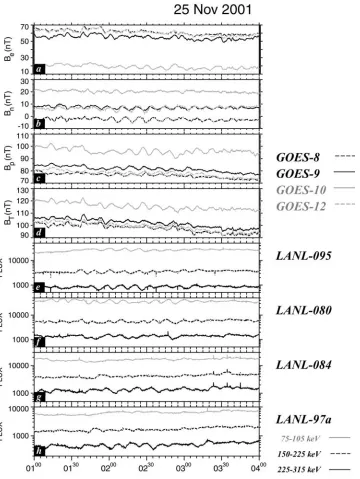
[18] Figures 7a – 7d shows the geosynchronous GOES -8,

-9, -10, and -12 magnetic field data in local spacecraft coordinates such that e is directed radially inward, n is azimuthally eastward (down-tail at dusk),pis parallel to the Earth’s spin axis, andtis the total magnetic field [Singer et al., 1996]. There are significant magnetic perturbations seen in all GOES spacecraft in all magnetic field components at

1.5 mHz frequency. The GOES-10 spacecraft observes significantly lower (by40 nT) radial Beand significantly

stronger (by15 nT) Bpand BTbackground magnetic field

strength as compared to GOES-8, -9, and – 12 and a larger azimuthal magnetic field strength. This is likely to be due to the fact that GOES-10 is closest to noon, while GOES-8, -9, and -12 are toward the nightside of the Earth and are in a more stretched magnetic field regime, thus with lower parallel and stronger earthward magnetic fields. The differ-ent magnetic latitudes of the spacecraft also contribute to the observed differences in the background fields. Indeed, these variations between GOES 10 and GOES -8, -9, and -12 have been confirmed by seeing similar variations in the Olson-Pfitzer 1977 quiet-time magnetic field model com-ponents at the GOES 8 and 10 locations. With regard to the waves, similar wave-packet structure (e.g., around 0140 – 0220 UT at GOES-10) appears in all the GOES satellites in the azimuthal Bncomponent. The azimuthal magnetic field

oscillations are first observed by GOES-10, then -9, -12, and finally GOES-8. Relating this to the spacecraft locations indicates the down-tail propagation of the magnetic distur-bances that excite this toroidal mode wave-packet. Figure 7d shows the total magnetic field from each of the four spacecraft. The compressional component of the wave can still be seen to some extent with the largest amplitudes in GOES-10, though the total magnetic fields do not change significantly (dB/B < 10%). The compressional wave com-ponent is most obvious in GOES-10, closest to noon, whereas the transverse component of the wave magnetic field is most obvious in GOES-8, -9, and -12, which are closer to midnight. Interestingly, the phase lag observed between satellites in the compressional component BT

(expected to be also classified by Bp and Be at this local

time) in this wave-packet appears to be much less than seen in Bn, although the same general phase lag trend (i.e.,

GOES-10, -9, -12, and -8) is apparent especially in Bp.

Comparing the phase variation of the azimuthal Bn

com-ponent between spacecraft pairs gives azimuthal wave numbers of m 1.3 – 6.5, propagating downtail, which is consistent with these perturbations being global-scale phenomena.

[19] Figures 7e – 7h shows LANL spacecraft observations

of electron fluxes in three energy channels, taken to be representative of the entire range of energy channels from the SOPA instrument. At 0200 UT, LANL-095 (at 2330 LT), LANL-080 (at 1500 LT), LANL-084 (at 0900 LT), and LANL-97a (at 0700 LT) provided information on the dawn, afternoon, and midnight sector geosynchronous particle populations. Interestingly, Figures 7e – 7h show that the geosynchronous electron fluxes are also being modulated at 1.4 – 1.6 mHz at all four LANL satellites. Significantly, the signatures in the electron fluxes at geosynchronous orbit are modulated much more strongly than the ions (not shown).

3.5. Ground-Based and Ionospheric Measurements

[20] The dusk sector of the magnetosphere is well

pop-ulated with ground-based instrumentation in this interval, and we use this instrumentation to characterize a well-defined field line resonance (FLR). In Table 1 we list the locations of the relevant CANOPUS magnetometer stations. Figure 8a shows the unfiltered H-component magnetic field measurements from the CANOPUS ‘‘Churchill line’’ from 0100 to 0400 UT on 25 November 2001. Data from the two highest-latitude Churchill line stations (TALO and RANK) were not available during this period. There is obvious large-amplitude and very narrow-band Pc5 ULF wave activity throughout the period, the clearest waves occurring between 0200 and 0300 UT, and the largest amplitudes occurring at the Gillam station.

[21] The H- (diamonds) and D- (stars) components were

[22] Comparing the phase variation of the longitudinally

separated station pair of FSI-FCH gives a maximum azimuthal wave number of m +4, i.e., propagating down-tail, and consistent with these waves being global magnetospheric phenomena in this event.

[23] Further evidence of the global nature of these

perturbations is shown by small-amplitude waves in the H-component magnetic perturbations observed by the SAMNET and IMAGE magnetometer arrays in the European sector (not shown). Referring to Figure 1, at

Figure 7. Geosynchronous magnetic field and electron observations from the GOES and LANL spacecraft, respectively. From top to bottom, (a) radial, (b) azimuthally eastward (downtail in this case), and (c) nearly field-aligned components of the magnetic field, together with (d) total magnetic field strength from the GOES-8, -9, -10, and -12 spacecraft. The geosynchronous electron fluxes are shown for three energy channels from the SOPA instrument, taken as representative for the interval for (e) LANL-095, (f) LANL-080, (g) LANL-084, and (h) LANL-97a.

Table 1. Coordinates of the CANOPUS Churchill Line and Selected SAMNET Magnetometer Stations Used in this Study

Station Code Geo. Lat. Geo. Lon. CGM Lat. CGM Lon.

0200 UT, the SAMNET array is situated around 0200 – 0300 MLT and the IMAGE array is situated 0400 – 0600 MLT. These measurements provide clear evidence for small-amplitude 1.4 – 1.6 mHz activity on the ground also being present in the predawn sector.

[24] Figure 9 shows the SuperDARN HF radar

mea-surements from six of the northern hemisphere radars between 1800 UT on 24 November 2001 and 0400 UT on 25 November 2001 in AACGM coordinates [Baker and Wing, 1989]. The color scales are independently scaled for each radar panel to accentuate the wave observation, though in all panels, blue denotes line-of-sight Doppler velocities toward the radar and red denotes line-of-sight velocities away from the radar. The dashed black and white line denotes the approximate location of local dusk at each radar bore site. Local dusk is around 0430 UT at Kodiak. Data were not available from the two radars at Hankasalmi and Pykkvibaer. Only one beam is shown from each of the radars for brevity, but data from these beams are represen-tative of essentially the entire radar field of views. Data from each beam shown in Figure 9 shows clear oscillations of the ionospheric line-of-sight velocity. There is also some poleward phase propagation of this backscatter in several beams, most notably in Prince George beam 6 (Figure 9b). However, most of the radar backscatter is too far poleward to see the FLR directly. The radars in the Alaskan sector

observed the ionospheric signatures at the lowest latitudes, which were possibly the signature of the FLR directly.

[25] Pc5 oscillations with a frequency of 1.4 mHz are

very clear just predusk in the0200 – 0300 UT period for the Prince George radar, in the latitude range 66 – 75°. Evidence for waves of similar frequency (1.5 mHz) can also be seen in the near range gates Kodiak in the same UT interval which corresponds to 64 – 73° and at higher lati-tudes in the 0100 – 0200 UT interval (73 – 75°). Back-scatter is generally poor for the Saskatoon and Kapuskasing radars between 0100 and 0400 UT during our wave interval, although evidence of 1.5 mHz waves is apparent in the Saskatoon radar around 69 – 72° in the period before it

0000 – 0150 UT, and at a much higher frequency in Kapuskasing around 66 – 70° between 2230 and 0100 UT in the 2.1 mHz range. These two radars are those conjugate to the Polar satellite and the CANOPUS Churchill line magnetometers. It must be stressed that the UT interval where the Kapuskasing radar has sufficient backscatter to observe ULF wave activity is not the same period as the principal wave event studied in this paper. Further east, the Goose Bay radar observes Pc5 waves between67 and 74°

in the 0130 – 0240 UT interval with a frequency of

1.3 mHz, which is similar to those seen at Polar and CANOPUS. Further east still, Iceland West saw wave activity in this broad frequency range (1.3 mHz) for

a very long time interval from 2000 to 0000 UT on 24 November 2001, however, backscatter is lost from around 0100 UT on 25 November onward.

[26] Interestingly, the ionospheric velocity oscillations for

each radar all occur within 5 hours of local dusk, this being evidence of similar ULF activity in the 1.4 – 1.6 mHz Pc5 range near or past dusk from 2000 UT on 24 November until around 0300 UT on the 25 November. Measurements of conjugate radar flows from Saskatoon and Kapuskasing with similar frequencies as those seen by Polar and CANOPUS

in the 0100 – 0400 UT interval are lacking, mostly due to loss of backscattered power. However, the adjacent Prince George and Goose Bay radars provide evidence that the same wave exists over an extended longitudinal range around dusk and in the 0100 – 0300 UT time interval.

4. Discussion

[27] The data presented in this paper provide very clear

evidence for an observational link between wave activity at

the magnetopause, in the magnetosphere, and in the iono-sphere, demonstrating the transport of solar wind energy through the near-Earth space environment with ULF waves. The first link in the chain of energy transfer between the solar wind and the ionosphere is observed by Cluster. We interpret the magnetic field and ion variations seen at Cluster to be due to the oscillatory motion of the topause boundary layer across the spacecraft. This magne-topause boundary motion can lead to the excitation of ULF waves inside the magnetosphere.

[28] Wright and Rickard[1995] produced numerical

sim-ulations that indicated in some cases global pulsations due to magnetospheric waveguide modes can be excited via buffeting at the magnetopause by the solar wind. In their studies these authors developed simulations of two solar wind drivers: a ‘‘stationary pulse,’’ characteristic of impulses over the magnetopause nose, which produced pulsations characteristic of the magnetosphere structure (independent of the pulse characteristics); and ‘‘running pulses,’’ expected to be characteristic of Kelvin-Helmholtz surface waves as well as moving magnetopause indenta-tions, which produced magnetopause ripples and hence waveguide modes and FLRs that had phase velocities equal to the speed of the running pulse.

[29] Rostoker and Sulivan [1987] found that 75% of

afternoon sector pulsations were associated with solar wind impulses. Mathie and Mann [2000] discussed the occurrence of observations of morning sector Pc5 FLRs with respect to sudden impulse events occurring in the solar wind, separating those associated with magneto-pause instabilities and those perhaps associated with sudden impulse events. These authors showed that for higher solar wind speeds, there was a clear correlation between the existence of common azimuthal phase speed multiple discrete frequency FLRs and the presence of high magnetosheath flow speed (>500 km s 1_{), which is}

consistent with Kelvin-Helmholtz magnetopause activity driving these discrete frequency waveguide modes which then drive FLRs [e.g., Mann et al., 1999]. Impulsive FLR excitation on the other hand was shown to be able to occur under any conditions, though mainly for lower solar wind speeds (<500 km s 1).

[30] Kepko et al. [2002] presented an interval where

there were discrete frequencies in the upstream solar wind number density and dynamic pressure, which correlated well with time-shifted observed magnetic field magnitude variations observed in the magnetosphere by the GOES spacecraft. These authors suggest that features inherent in the solar wind at discrete frequencies may be responsible for discrete frequency global ULF pulsations in the magnetosphere.

[31] The data collected at Polar, located in the dusk

sector central plasma sheet around L 9, shows an Alfve´n wave signature of 4 nT peak-to-peak magnetic and 2 mVm 1 peak-to-peak electric field amplitude which persists for 2.5 hours in the data set. Our analysis has shown that this wave is predominantly a standing transverse Alfve´n wave with a significant field-aligned component of the Poynting vector. Given that the Polar observations are made near the equatorial plane, the proximity of Polar to the expected equatorial node may explain the significantly smaller magnetic amplitude seen

at Polar as compared to CANOPUS on the ground. This interpretation is also supported by the2 mV m 1 peak-to-peak electric field amplitude. The data from Polar also shows there is a small compressional magnetic compo-nent to this wave, which may represent the driving fast compressional waveguide mode. The fact that there is still compressional wave activity present around this region is further verified by the magnetic field measurements by the GOES spacecraft. The azimuthal component of the Poynting vector of the wave as determined by the Polar data has a large contribution from the compressional component and is directed antisunward, which is consis-tent with compressional waveguide modes driven by magnetopause fluctuations which propagate antisunward downtail in the Earth’s magnetospheric waveguide. The small amplitude of the compressional magnetic field component (expected to have an antinode in the equato-rial plane) may result from the fact that the driving compressional waveguide mode energy density is spread globally throughout the outer magnetospheric waveguide. Alternately, the driving fast mode source could be an evanescent magnetopause surface mode [e.g., Southwood, 1974] rather than by Kelvin-Helmholtz excited overre-flected body-type waveguide modes [e.g., Mann et al., 1999].

[32] We postulate that the wave energy is most probably

generated by a Kelvin-Helmholtz type instability on the magnetopause driving compressional waves traveling in-ward through the magnetosphere. Some of this energy is then transferred to standing Alfve´n waves along field lines in a region that brackets the GOES and PolarLshells (L

6 – 9). Both SuperDARN radar data and ground-based magnetometer networks observe these standing waves. All of the waves observed have a clearly defined quasi-stable central frequency in the range 1.4 – 1.6 mHz, based on which we argue that these waves are clearly are part of a well-defined path of energy transfer from the solar wind driven magnetopause oscillations to the inner magneto-sphere and ionomagneto-sphere.

[33] The discrete frequency signatures seen by the

ground-based CANOPUS array and by Polar in situ in the magnetosphere are also observed magnetically by the four GOES spacecraft situated approximately between local noon and local dusk, as well as via energetic electron signatures on four LANL satellites distributed from approx-imately midnight to the postnoon sector. The LANL elec-tron data show clearer oscillations in the 225 – 315 keV energy channel for the SOPA throughout these local times, although it is also seen in the lower-energy 150 – 225 keV and 75 – 105 keV channels, especially at LANL-095 and -080. Although the phase relationships between the fluxes in different energy channels at different LANL spacecraft seem to be complex, it seems clear that the energetic electrons are coupled to the discrete frequency ULF wave. The global nature of the electron flux variations suggests that local interactions between the monochromatic duskside FLR electric field and the energetic electrons produced effects along the drift-path which is observed at other local times by the LANL satellite constellation at each satellite location.

[34] Mann et al.[2002] showed that during one fast solar

with a frequency of 2 – 2.5 mHz, which in turn drove discrete frequency FLRs believed to have been driven by Kelvin-Helmholtz unstable magnetospheric waveguide modes. However, during this interval, there were no space-craft in and around the mode-conversion region. In contrast, in this study the Polar spacecraft provides key information about the mode-conversion region and yields stronger insights into the energy transfer process during the interval presented here.

[35] An important aspect of our data analysis for this

event is the calculation of the wave Poynting vector from the Polar electric and magnetic fields. We find that there is a very small radial, significant azimuthal, and dominant field-aligned component to the wave Poynting vector. In a similar study,Clemmons et al.[2000] presented Polar observations of several wave cycles of electric and magnetic Pc5 activity during a magnetic cloud driven event in the magnetosphere. These authors also determined that the ULF waves had significant field-aligned component of the Poynting vector and concluded that this was due to two counterpropagating (toroidal and poloidal polarization) shear Alfve´n waves which had pulsation signatures characteristic of FLRs on the ground. In contrast, for the study presented here we offer the simple interpretation that the large oscillatory Poynting vectors we observed were standing mode shear Alfve´n waves set up along the resonant field line situated close to the orbital location of Polar.

[36] The interval presented in this paper is remarkable for

a number of reasons. For energy and momentum to be traced from solar wind, into the terrestrial environment, and down into the ionosphere and the ground demands a favorable conjunction of satellite and ground instrumenta-tion. Several studies have carried out analysis of some of the steps in this pathway of energy transfer, but ours is the first such interval to have spacecraft in all relevant areas and ground-based coverage to track energy transfer from the magnetopause down to the Earth’s surface.

[37] Perhaps more importantly, our observations provide

evidence that discrete frequency waveguide modes and FLRs can be excited by K-H shear flow instability at the magnetopause [Mann et al., 1999; Mills et al., 1999]. As discussed by Mann et al. [1999], for magnetosheath flow speeds greater than a critical value (500 km s 1) Kelvin-Helmholtz instabilities at the magnetopause can couple to body-type waveguide modes. In this case these discrete frequency waveguide modes can be excited by K-H shear-flow instability at the magnetopause. It should be noted that the classic KH surface wave instability, excited at a boundary between two semi-infinite media, has an upper cutoff flow speed beyond which the KH surface mode is no longer unstable. In the case where the one of media is bounded (in this case the magnetosphere) low-m body-type waveguide modes do not possess a maximum flow speed for instability; rather, in order to excite the body-type modes, the flow speed must be greater than a critical speed in order for shear flow K-H instability to generate growing modes (see Mann et al. [1999] and Mills et al. [1999] for more details). We believe that the discrete frequency Pc5 FLR reported here was excited by this mechanism.

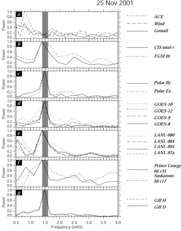
[38] Finally, we present a spectral analysis of the

time-shifted (by 24 min) solar wind dynamic pressure, together

with data from each spacecraft and instrument from this interval. The parameters shown here are taken as represen-tative, as there is simply too much information presented in this paper to show all parameters at each location. Figure 10 shows a composite plot of solar wind dynamic pressure (Figure 10a), Cluster magnetic fields and plasma measure-ments close to the magnetopause (Figure 10b), transverse magnetospheric magnetic and electric fields from Polar (Figure 10c), azimuthal magnetospheric fields (Figure 10d), geosynchronous electron fluxes (Figure 10e), ionospheric line-of-sight velocities (Figure 10f), and ground magnetic perturbations (Figure 10g). The grey area denotes the 1.4 – 1.6 mHz band. From Figure 10 we can see that no spectral peak is apparent in the appropriately lagged solar wind dynamic pressure in this frequency band, whereas there are dominant spectral peaks in Figures 10b – 10g in the magnetospheric and ionospheric magnetic fields and veloc-ities, magnetospheric electric fields, and particle fluxes. From this we conclude that the magnetospheric and iono-spheric oscillations are not related to the action of direct driving by solar wind dynamic pressure variations, such as those outlined byKepko et al.[2002].

5. Conclusions

[39] In summary, we present observations from 2

waveguide, while the energy originates from boundary oscillations at the magnetopause.

[40] The excellent conjunction of ground- and

space-based instrumentation in the afternoon sector provides a means to trace energy from the solar wind into the Earth’s magnetosphere and ionosphere. Few studies have identi-fied a one-to-one correspondence between magnetopause oscillations and ionospheric wave activity. In this event, the Polar data provides a direct link between Cluster

measurements of magnetopause oscillations and FLR signatures detected in the ionosphere by SuperDARN and the CANOPUS magnetometer network. This is the first such study to have such advantageous instrumentation collecting data over the same time interval.

[41] Our observations are consistent with the hypothesis

that Kelvin-Helmholtz instability at the magnetopause ex-cited discrete frequency compressional waveguide modes in the magnetosphere. These waveguide modes propagated

Figure 10. Normalized FFT power spectra of (a) time-lagged (24 min) solar wind dynamic pressure, (b) Cluster-3 total magnetic field and total ion velocity (c) Polar Ex and By measurements in

downtail and excited a large-amplitude discrete frequency field line resonance in the dusk local time sector.

[42] Acknowledgments. The authors would like to thank R. Lepping and K. Ogilvie of Goddard Space Flight Center for the use of Wind MFI and SWEPAM data. ACE data were provided by CDAWeb and by Ruth Skoug and the ACE/SWEPAM team. The CANOPUS instrument array (now CARISMA http://www.carisma.ca) constructed, maintained, and operated by the Canadian Space Agency provided the data used in this study. We would like to thank C. T. Russell for use of the Polar MFE data and for helpful discussions, and F. S. Mozer for Polar EFI data under NASA grant NAG5-11733. F.R.F., E.F.D., C.E.J.W, and I.R.M are funded by the Natural Sciences and Engineering Research Council of Canada (NSERC). I.J.R. is funded by NSERC and the Canadian Space Agency (CSA). During part of the preparation of this manuscript ML was at the Institute for Advanced Study, La Trobe University, Melbourne.

[43] Arthur Richmond thanks the reviewers for their assistance in evaluating this paper.

References

Acuna, M. H., K. W. Ogilvie, D. N. Baker, S. A. Curtis, D. H. Fairfield, and W. H. Mish (1995), The Global Geospace Science program and its in-vestigations,Space Sci. Rev.,71, 5 – 21.

Allan, W., S. P. White, and E. M. Poulter (1986), Impulse-excited hydro-magnetic cavity and field line resonances in the magnetosphere,Planet. Space Sci.,34, 371.

Allan, W., E. M. Poulter, and J. R. Manuel (1990), Does the ponder-omotive force move mass in the magnetosphere?,Geophys. Res. Lett., 17, 917.

Anderson, B. J., M. J. Engebretson, S. P. Rounds, L. J. Zanetti, and T. A. Potemra (1990), A statistical study of Pc3 – Pc5 pulsations observed by the AMPTE/CCE magnetic fields experiment: 1. Occurrence distribu-tions,J. Geophys. Res.,95, 10,495.

Baker, K. B., and S. Wing (1989), A new magnetic coordinate system for conjugate studies at high latitudes,J. Geophys. Res.,94, 9139. Balogh, A., et al. (1997), The Cluster Magnetic Field experiment,Space

Sci. Rev.,79, 65.

Beamish, D., H. Hanson, and D. Webb (1979), Complex demodulation applied to Pi2 geomagnetic pulsations,Geophys. J. R. Astron. Soc.,58, 471.

Belian, R. D., G. R. Gisler, T. E. Cayton, and R. Christensen (1992), High Z energetic particles at geosynchronous orbit during the great solar proton event of October, 1989,J. Geophys. Res.,97, 16,897.

Chen, L., and A. Hasegawa (1974), A theory of long-period magnetic pulsations: 1. Steady state excitation of field line resonance,J. Geophys. Res.,79, 1033.

Chiu, M. C., et al. (1998), ACE spacecraft,Space Sci. Rev.,86, 257. Clemmons, J. H., et al. (2000), Observations of traveling Pc5 waves and

their relation to the magnetic cloud event of January 1997,J. Geophys. Res.,105, 5441.

Dungey, J. W. (1955), Electrodynamics of the outer atmosphere, in Proceedings of the Ionosphere, p. 255, Phys. Soc. of London, London. Elkington, S. R., M. K. Hudson, and A. A. Chan (1999), Acceleration of relativistic electrons via drift-resonant interaction with toroidal-mode Pc5 ULF oscillations,Geophys. Res. Lett.,26, 3273.

Fenrich, F. R., and J. C. Samson (1997), Growth and decay of field line resonances,J. Geophys. Res.,102, 20,031.

Greenwald, R. A., et al. (1995), Darn/Superdarn: A global view of the dynamics of high-latitude convection,Space Sci. Rev.,71, 761. Harvey, P., et al. (1995), The Electric Field Instrument on the Polar satellite,

Space Sci. Rev.,71, 583.

Hughes, W. J., and D. J. Southwood (1976), The screening of micropulsa-tion signals by the atmosphere and ionosphere,J. Geophys. Res.,81, 3234.

Kepko, L., H. E. Spence, and H. J. Singer (2002), ULF waves in the solar wind as direct drivers of magnetospheric pulsations,Geophys. Res. Lett., 29(8), 1197, doi:10.1029/2001GL014405.

Khan, H., and S. W. H. Cowley (1999), Observations of the response time of high-latitude ionospheric convection to variations in the inter-planetary magnetic field using EISCAT and IMP-8 data, Ann. Geo-phys., 17, 1306.

Kivelson, M. G., and D. J. Southwood (1985), Resonant ULF waves: A new interpretation,J. Geophys. Res.,12, 49.

Kivelson, M. G., J. Etcheto, and J. G. Trotignon (1984), Global compres-sional oscillations of the terrestrial magnetosphere: The evidence and a model,J. Geophys. Res.,89, 9851.

Lepping, R. P., et al. (1995), The Wind magnetic field investigation,Space Sci. Rev.,71, 207.

Lessard, M. R., M. K. Hudson, and H. Lu¨hr (1999a), A statistical study of Pc3-Pc5 magnetic pulasations observed by the AMPTE/Ion Release Module satellite,J. Geophys. Res.,104, 4253.

Lessard, M. R., M. K. Hudson, J. C. Samson, and J. R. Wygant (1999b), Simultaneous satellite and ground-based observations of a discretely dri-ven field line resonance,J. Geophys. Res.,104, 12,361.

Lotko, W., A. V. Streltsov, and C. W. Carlson (1998), Discrete auroral arc, electrostatic shock and suprathermal electrons powered by dispersive, anomalously resistive field line resonances, Geophys. Res. Lett.,25, 4449.

Mann, I. R., A. N. Wright, K. J. Mills, and V. M. Nakariakov (1999), Excitation of magnetospheric waveguide modes by magnetosheath flows, J. Geophys. Res.,104, 333.

Mann, I. R., et al. (2002), Co-ordinated ground-based and Cluster observa-tions of large amplitude global magnetospheric oscillaobserva-tions during a fast solar wind speed interval,Ann. Geophys.,20, 405.

Mathie, R. A., and I. R. Mann (2000), Observations of Pc5 field line resonance azimuthal phase speeds: A diagnostic of their excitation mechanism,J. Geophys. Res., 105, 10,713.

McComas, D. J., S. J. Bame, P. Barker, W. C. Feldman, J. L. Phillips, P. Riley, and J. W. Griffee (1998), Solar Wind Electron Proton Alpha Monitor (SWEPAM) for the Advanced Composition Explorer, Space Sci. Rev., 86, 561.

Mills, K. J., A. N. Wirght, and I. R. Mann (1999), Kelvin-Helmholtz driven modes of the magnetosphere,Phys. Plasmas.,6, 4070.

Miura, A. (1987), Simulation of Kelvin-Helmholtz instability at the mag-netospheric boundary,J. Geophys. Res.,92, 3195.

Ogilvie, K. W., et al. (1995), SWE, a comprehensive plasma instrument for the WIND spacecraft,Space Sci. Rev.,71, 55.

Peredo, M., J. A. Slavin, E. Mazur, and S. A. Mazur (1995), 3-dimensional position and shape of the bow shock and their variation with Alfvenic, sonic, and magnetosonic Mach number and interplanetary magnetic-field orientation,J. Geophys. Res.,100, 7907.

Re`me, H., et al. (2001), First multispacecraft ion measurements in and near the Earth’s magnetosphere with the identical Cluster ion spectrometry (CIS) experiment,Ann. Geophys.,19, 1303.

Rostoker, G., and B. T. Sulivan (1987), Polarisation characteristics of Pc5 magnetic pulsations in the dusk hemisphere, Planet. Space Sci., 35, 429.

Rostoker, G., J. C. Samson, F. Creutzberg, T. J. Hughes, D. R. McDiarmid, A. G. McNamara, A. Vallance Jones, D. D. Wallis, and L. L. Cogger (1995), CANOPUS - A ground based instrument array for remote sensing the high latitude ionosphere during the ISTP/GGS program,Space Sci. Rev.,71, 743.

Russell, C. T., R. C. Snare, J. D. Means, D. Pierce, D. Dearborn, M. Larson, G. Barr, and G. Le (1995), The GGS/Polar magnetic fields investigation, Space Sci. Rev.,71, 563.

Samson, J. C., J. A. Jacobs, and G. Rostoker (1971), Latitude dependent characteristics of long period geomagnetic micropulsations,J. Geophys. Res.,76, 3675.

Samson, J. C., B. G. Harrold, J. M. Ruohoniemi, and A. D. M. Walker (1992a), Field line resonances associated with MHD waveguides in the magnetosphere,Geophys. Res. Lett.,19, 441.

Samson, J. C., D. D. Wallis, T. J. Hughes, F. Creutzberg, J. M. Ruohoniemi, and R. A. Greenwald (1992b), Substorm intensifications, and field line resonances in the nightside magnetosphere,J. Geophys. Res.,97, 8495. Shue, J. H., J. K. Chao, H. C. Fu, C. T. Russell, P. Song, K. K. Khurana, and H. J. Singer (1997), A new functional form to study the solar wind control of the magnetopause size and shape,J. Geophys. Res.,102, 9497. Singer, H. J., L. Matheson, R. Grubb, A. Newman, and S. D. Bouwer (1996), Monitoring space weather with the GOES magnetometers,SPIE Proc.,2812, 299 – 308.

Smith, C. W., J. L’Heureux, N. F. Ness, M. H. Acuna, L. F. Burlaga, and J. Scheifele (1998), The ACE magnetic fields experiment,Space Sci. Rev.,86, 611.

Southwood, D. J. (1974), Some features of field line resonances in the magnetosphere,Planet. Space Sci.,22, 483.

Southwood, D. J., J. W. Dungey, and R. L. Etherington (1969), Bounce resonant interaction between pulsations and trapped particles, Planet Space Sci.,17, 349.

Tsyganenko, N. A. (1989), A magnetospheric magnetic field model with a warped tail current sheet,Planet. Space Sci.,37, 5.

Walker, A. D. M. (1981), The Kelvin-Helmholtz instability in the low-latitude boundary layer,Planet. Space Sci.,829, 1119.

Walker, A. D. M., R. A. Greenwald, W. F. Stuart, and C. A. Green (1979), STARE auroral radar observations of Pc5 geomagnetic pulsations, J. Geophys. Res.,84, 3373.

Wright, A. N. (1994), Dispersion and wave coupling in inhomogenous MHD waveguides,J. Geophys. Res.,99, 159.

Wright, A. N., and G. J. Rickard (1995), ULF pulsations driven by mag-netopause motions: Azimuthal phase characteristics,J. Geophys. Res., 101, 24,991.

Yeoman, T. K., D. K. Milling, and D. Orr (1990), Pi2 pulsation patterns on the UK Sub-Auroral Magnetometer Network, Planet. Space Sci., 38, 589.

A. Balogh, Physics Department, Imperial College London, London SW7 2 AK, UK.

E. F. Donovan, Department of Physics and Astronomy, University of Calgary, Calgary, Alberta TN2 1N4, Canada.

F. R. Fenrich, I. R. Mann, D. K. Milling, I. J. Rae, and C. E. J. Watt, Department of Physics, University of Alberta, Edmonton, Alberta T6G 2J1, Canada. ( [email protected])

B. Lavraud, Los Alamos National Laboratory, MS D436, Los Alamos, NM 87545, USA.

M. Lester and J. A. Wild, Department of Physics and Astronomy, University of Leicester, Leicester LE1 7RH, UK.

H. Re`me, Centre d’Etude Spatiale des Rayonnements, BP 4346, 9 Ave Colonel Roche, Cedex, Toulouse F-31029, France.