Optimal control, self tuning techniques and their application to dynamically positioned vessels

Optimal control, self-tuning techniques and their

application to dynamically positioned vessels

FUNG, Patrick Tze-Kwai

Available from Sheffield Hallam University Research Archive (SHURA) at:

http://shura.shu.ac.uk/7119/

This document is the author deposited version. You are advised to consult the

publisher's version if you wish to cite from it.

Published version

FUNG, Patrick Tze-Kwai (1983). Optimal control, self-tuning techniques and their

application to dynamically positioned vessels. Doctoral, Sheffield City Polytechnic.

Copyright and re-use policy

P O L Y T E C H N IC L I3 R A R Y | | P O N D S T R E E T

SH EFFIELD S I 1W B

OPTIMAL CONTROL, SELF-TUNING TECHNIQUES AND THEIR APPLICATIONS TO DYNAMICALLY POSITIONED VESSELS

Patrick T K Fung

ABSTRACT

This thesis consists of two parts. The development of a self-adaptive stochastic control system for dynamically positioned vessels is described in Part One. Part Two is the investigation and the development of self-tuning control techniques.

In Part One, the dynamic ship positioning control problems and basic components are described. The modelling techniques of low frequency ship motions and wave motions are given. The various Kalman filtering methods are appraised. An optimal state feedback control with integral action for the ship positioning system is proposed, followed by the

simplification of the complex control structure to allow easy implementation. A self-tuning Kalman filter is proposed for systems which have low frequency outputs corrupted by high frequency disturbances. This filter is used in the ship positioning system. Simulation results of scalar, multivari­ able and non-linear cases are given.

Part Two begins with the development of an adaptive tracking technique for slowly varying processes with coloured noise disturbances. Estimated results for various wave signals are given. The self-tuning control techniques are overviewed,

followed by the development of an explicit multivariable weighted minimum variance controller. Simulation results

including the estimation of system time delay are given. Finally, an implicit weighted minimum variance controller for single input-single output system is developed.

ProQuest Number: 10694093

All rights reserved INFORMATION TO ALL USERS

The quality of this reproduction is dependent upon the quality of the copy submitted. In the unlikely event that the author did not send a com plete manuscript and there are missing pages, these will be noted. Also, if material had to be removed,

a note will indicate the deletion.

uest

ProQuest 10694093

Published by ProQuest LLC(2017). Copyright of the Dissertation is held by the Author. All rights reserved.

This work is protected against unauthorized copying under Title 17, United States C ode Microform Edition © ProQuest LLC.

ProQuest LLC.

789 East Eisenhower Parkway P.O. Box 1346

OPTIMAL CONTROL, SELF-TUNING TECHNIQUES AND THEIR APPLICATIONS TO DYNAMICALLY POSITIONED VESSELS

by

PATRICK TZE-KWAI FUNG

A thesis submitted to the Council For

National Academic Awards in partial fulfillment of the requirements for the degree of

Doctor of Philosophy

The research was conducted at Sheffield City Polytechnic in collaboration with GEC Electrical

Projects Ltd., Rugby

DECLARATION

This is to declare that the author, while regis­ tered as a candidate for the degree for which the submission of this thesis is made, has not been a registered candidate for another award of CNAA or of a university during the research program.

(P.T.K. Fung) v

-i-0/5/mcla704/3

0/5/mcla704/4

ACKNOWLEDGEMENTS

The work presented in this thesis was basically completed at the end of 1981. However, a series of exciting events

happened thereafter: the removal of the research team from Sheffield City Polytechnic to the University of Strathclyde? the coming of the author's daughter to his family; immigra­ tion to Canada and taking up a new appointment at Spar Aerospace. The author is indebted to Professor Mike

J. Grimble for his encouragement, inspiration and guidance throughout the project, particularly for his patience to this belated presentation.

The author would also like to express his sincere gratitude to the following:

Dr. P.J. Gawthrop, for his advice on self-tuning techniques.

Mr. D. Wise and Mr. P. Urry, for their technical supervision.

Dr. T.J. Moir and Dr. A. Al-Takie for their helpful discus­ sions throughout the research work.

0/5/mcla704/5

Mrs. P. Cheung, the author's Godmother, for her support and encouragement during his study in Britain.

British Science and Engineering Research Council, for their financial support of the project.

GEC Electrical Projects Ltd., for their technical support of the project on dynamic ship positioning.

Department of Electrical and Electronic Engineering of Sheffield City Polytechnic and of the University of

Strathclyde, for providing the facilities for the research work.

Spar Aerospace Ltd., RMS Division, for providing the typing facility.

Mrs. Cathy Nowik, Mrs. Cathy Atkins and Barbara Parkin for their excellent typing of a difficult manuscript.

0/5/mcla704/6

C O N T E N T S

Page

ACKNOWLEDGEMENTS i i i

ABSTRACT xiv

CONTRIBUTIONS AND PUBLICATIONS xvi

INTRODUCTION xx

PART I

CHAPTER ONE DYNAMIC SHIP POSITIONING SYSTEM 1

1.1 Introduction 1

1.2 Control Problems 2

1.3 Basic Components 5

1.3.1 Sonar Measurement

System 5

1.3.2 Taut Wire Measurement

System 8

1.3.3 Radio Measurement

System 8

1.3.4 Thrusters 11

1.3.5 Wind Speed/Direction

Measurement System 11

CHAPTER TWO DYNAMIC MODELLING OF VESSEL MOTIONS 14

2.1 The Motions of Vessels 14

2.2 The Non-Linear Low Frequency Ship

Model 17

2.3 The Linearized Low Frequency Ship

Model 19

-v-0/5/mcla704/7

Contents (continued) Page

2.4 Thruster Allocation Logic 21

2.5 The Non-Linear Thruster Model 22

2.6 The Linear Thruster Model 29

2.6.1 First Order

Approximation 29

2.6.2 Second Order

Approximation 29

2.7 The Dynamic Models of Wimpey

Sealab 30

2.7.1 The Low Frequency Model 32

2.7.2 The Noise Covariance

Specifications 37

2.8 High Frequency Models 38

2.8.1 Rational Proper

Transfer Function Model 39

2.8.2 Auto-Regressive Moving

Average Model 45

2.8.3 Harmonic Oscillation

Model 46

2.8.4 Simulation of High

Frequency Motions 48

vi-0/5/mcla704/8

Contents (continued) Page

2.9 The Linear State Space Equations for Ship Motions

CHAPTER THREE THE KALMAN FILTERING PROBLEMS OF DYNAMIC SHIP POSITIONING SYSTEMS

3.1 The Estimation Structure

3.2 Extended Kalman Filter Using Harmonic Wave Model

3.3 Constant Gain Linear Kalman Filter

3.4 Extended Kalman Filter Using Four Order Wave Models

CHAPTER FOUR THE STOCHASTIC OPTIMAL CONTROL PROBLEM IN DYNAMIC POSITIONING SYSTEMS

4.1 Introduction

4.2 Optimal Controller Design Philosophy

4.3 Optimal Controller with Integral Action

49

52

52

55

59

60

61

61

61

63

65

-vii-0/5/mcla704/9

Contents (continued)

4.3.1 System Description

4.3.2 Optimal Regulating

Problem

4.3.3 Control Problem

4.3.4 Filtering Problem

4.3.5 Stability of Closed

Loop Output Feedback System

4.3.6 Implementation on the

Dynamic Ship

Positioning System

4.4 Simplified DP Integral Control Systems

4.4.1 System Models

4.4.2 Control System Design

One and Simulation Results

4.4.3 Control System Design

Two and Simulation Results

4.4.4 Control System Design

0/5/mcla704/l0

Contents (continued)

4.5 Summary of Results

CHAPTER FIVE THE SELF-TUNING KALMAN FILTER

5.1 Introduction

5.2 The System Description 5.3 The Low Frequency Motion

Estimator

5.4 The High Frequency Motion Estimator

5.5 Modified Estimation Equations 5.6 Kalman and Self-Tuning Filter

Algorithms 5.7 Discussion

5.8 Summary of Results

CHAPTER SIX THE USE OF SELF-TUNING KALMAN FILTERING

TECHNIQUES IN DYNAMIC SHIP POSITIONING SYSTEMS

6.1 Introduction

6.2 Linear System Implementation

6.2.1 Single Input - Single

Output Systems

-ix-0/5/mcla704/ll

Contents (continued) Page

6.2.2 Multi Input - Multi

Output Systems 157

6.3 Non-linear System Implementation 175

6.4 Self-Tuning Kalman Filter with

Integral Control 189

6.5 Summary of Results 194

PART II

CHAPTER SEVEN THE ADAPTIVE TRACKING OF SLOWLY VARYING PROCESSES WITH COLOURED NOISE

DISTURBANCES 195

7.1 Introduction 195

7.2 System Description 196

7.3 Tracking and Filtering Problems 199

7.4 The Design of Adaptive Estimator 200

7.5 Simulation Results 206

7.6 Summary of Results 213

-x-0/5/mcla704/l2

Contents (continued) Page

CHAPTER EIGHT SELF-TUNING CONTROL AND WEIGHTED

MINIMUM VARIANCE SELF-TUNERS 214

8.1 Introduction 214

8.2 Self-Tuning Control Overview 214

8.2.1 The Self-Tuning Control 214

8.2.2 The Development 217

8.2.3 Implementation,

Advantages and

Disadvantages 222

8.3 Explicitly Multivariable Weighted Minimum Variance Self-Tuning

Controller 226

8.3.1 IntfoductionSystem 226

8.3.2 Description 227

8.3.3 The Cost Function 229

8.3.4 Multivariable Weighted

Minimum Variance

Controller 230

8.3.5 Explicit Self-Tuning

Control 234

-xi-0/5/mcla704/l3

Contents (continued) Page

8.3.6 Discussion 237

8.3.7 Industrial Applications 240

8.4 Implicit Weighted Minimum Variance

Self-Tuner 241

8.4.1 Introduction 241

8.4.2 Plant Description 241

8.4.3 Weighted Minimum

Variance Controller 243

8.4.4 Implicit Self-Tuning

Control 245

8.4.5 Discussion 251

CHAPTER NINE OVERALL CONCLUSIONS AND FUTURE WORK 252

9.1 Overall Conclusions 252

9.2 Future Work 254

-xii-0/5/mcla704/l4

Contents (continued) Page

REFERENCES 256

APPENDIX A TRANSFER FUNCTION WAVE MODELS FOR

VARIOUS SEA CONDITIONS 285

APPENDIX B WIMPEY SEALAB PER UNIT SYSTEM

SPECIFICATIONS 293

APPENDIX C DISCRETE KALMAN GAIN MATRIX

COMPUTATION 295

APPENDIX D A RECURSIVE ALGORITHM FOR SMOOTHING

AND PREDICTING OF A SIGNAL 298

APPENDIX E WEIGHTED MINIMUM VARIANCE CONTROLLER

DERIVATION 300

APPENDIX F PUBLISHED PAPER 307

-xiii-0/5/mcl704/l

OPTIMAL CONTROL, SELF—TUNING TECHNIQUES AND

THEIR APPLICATIONS TO DYNAMICALLY POSITIONED VESSELS

Patrick T K Fung

ABSTRACT

This thesis consists of two parts. The development of a self-adaptive stochastic control system for dynamically positioned vessels is described in Part One. Part Two is the investigation and the development of self-tuning control techniques.

In Part One, the dynamic ship positioning control problems and basic components are described. The modelling techniques of low frequency ship motions and wave motions are given. The various Kalman filtering methods are appraised. An optimal state feedback control with integral action for the

ship positioning system is proposed, followed by the simplification of the complex control structure to allow easy implementation. A self-tuning Kalman filter is proposed for systems which have low frequency outputs corrupted by high frequency disturbances. This filter is used in the ship positioning system. Simulation results of scalar, multivari­ able and non-linear cases are given.

Part Two begins with the development of an adaptive tracking technique for slowly varying processes with coloured noise disturbances. Estimated results for various wave signals are given. The self-tuning control techniques are overviewed,

0/5/mcl704/3

CONTRIBUTIONS AND PUBLICATIONS

Main Contributions

1. The developmment of the dynamic models and the analysis of the control design philosophy of ship positioning systems.

2. The analysis of the Kalman Filter problem and struc­ tures for ship positioning systems.

3. The development of stochastic optimal control systems including integral actions for dynamically positioned vessels.

4. The development of a self-tuning Kalman filter for sys­ tems with unknown high frequency disturbances.

5. The use of self-tuning Kalman filter for dynamically positioned vessels, which includes single input-single output, multivariable and non-linear cases.

6. The extension of the dynamic models for dynamic posi­ tioning control and filtering to include a second order linear thruster model.

-xvi-0/5/mcl704/4

7. The development of an adaptive tracking technique for slowly varying systems with coloured noise

disturbances.

8. The development of an explicit multivariable weighted minimum variance controller.

9. The development of an implicit single input-single output weighted minimum variance controller.

Publications

1. Fung, P.T.K. and Grimble M.J. 1981, "Self-Tuning Control of Ship Positioning Systems" IEE Workshop on Self-Tuning and Adaptive Control, March, Oxford

University, U.K. Also published by Peter Peregrinus Ltd. and edited by C.J. Harris and S.A. Billings.

0/5/mcl704/5

3. Grimble M.J. and Fung P.T.K. 1981 "Explicit Weighted Minimum Variance Self-Tuning Controllers" IEEE Conf. on Decision and Control, December, San Diego, Calif.,

U.S.A.

4. Grimble M.J. Johnson M.A. and Fung P.T.K. 1980 "Optimal Self-Tuning Control Systems: Theory and Application, Part I Introduction Controller Design", Trans. Inst. Measurement and Control, Vol. 2, No. 3, pll5-119.

5. Grimble M.J., Fung P.T.K. and Johnson M.A. 1982, "Optimal Self-Tuning Control Systems: Theory and Application, Part II, Identification and Self-Tuning" Trans. Inst. Measurement and Control, Vol. 4, No. 1, p25-36.

6. Grimble M.J. Moir T.J. and Fung P.T.K. 1982, "Compari­ son of WMV and LQG Self-Tuning Controllers", IEEE Symposium on Multivariable and Stochastic Control Theory, Hull, U.K.

7. Fung P.T.K., Chen Y.L. and Grimble M.J., 1982, "Dynamic Ship Positioning Control Systems Design Including

Non-linear Thrusters and Dynamics", NATO Advanced Study Institute on Non-linear Stochastic Problems, May,

Algarve, Portugal. Also published in "Nonlinear

i-0/5/mcl704/6

Stochastic Problems", NATO ASI series on Mathematical and Physical Sciences No. 104, Edited by R.C. Bucy and J.M.F. Moura, published by Reidel, 1983.

8. Fung P.T.K. and Grimble M.J. 1983 "Dynamic Ship Posi­ tioning Using a Self-Tuning Kalman Filter", IEEE Trans AC-28, No. 3, March, Special Issue on Applications of Kalman Filtering, p339-350.

9. Fung P.T.K. Chen X.P. and Grimble M.J. 1982", The Adaptive Tracking of Slowly Varying Processes with Coloured Noise Disturbances", Submitted Trans. Inst. Measurement and Control.

Reports

1. Fung P.T.K., 1980, "Optimal and Self-Tuning of Dynamically Positioned Vesels", Sheffield City Polytechnic Research Report, EEE/64.

0/5/mcl704/7

INTRODUCTION

Objectives

The contents of this thesis are separated into two main parts. Part I involves the solution of the dynamic ship positioning control problem using optimal and self-tuning techniques. This is the main theme of the thesis. Part II is concerned with the development of adaptive and self­

tuning control theory.

Introduction to Part I

The abundant deposits in the ocean seabed have become the targets for energy and mineral searches. The development is progressing towards deeper seas. Thence the demand for

technical support by way of dynamically positioned vessels is increasing and the performance specifications are becom­ ing tightened. Basically, the position control of a vessel must only allow for a maximum certain radial position

error. The control system must avoid high frequency fluctu­ ations in the thruster demands. Moreover, the controller must be capable of eliminating any offset due to constant disturbances.

-xx-0/5/mcl704/8

In the conventional dynamic system using Proportional- Inte­ gral-Derivative (PID) controllers and notch filters, the wave filter imposes a phase lag on the position error signals. This phase lag restricts the allowable bandwidth that can be used for the controller, whilst still

maintaining the stability margins required for satisfactory controller performance; hence an inevitable conflict arises between bandwidth and filter attenuation. The more effec­ tive the wave filter becomes in reducing the thruster oscil­ lations due to the waves, the more restriction is placed on the controller bandwidth and hence on the position holding accuracy. These considerations have led to the development of a second generation of dynamic positioning systems,

designed using optimal stochastic control theory and

employing the Kalman filter.

The non-linearity and the uncertainty of ship parameters and weather conditions are the main obstacles in achieving a good performance for the control system. The recent devel­ opment of the self-tuning control theory has encouraged the author to investigate the use of self-tuning techniques in dynamic ship positioning systems. Self-tuning of dynamical­ ly positioned vessels can be classified as the third

0/5/mcl704/9

Introduction to Part II

When the author was solving the dynamic ship positioning control problem, he was encouraged by Professor M.J. Grimble to work on self-tuning control as well. This attempt led to the development of a self-adaptive tracker for slow varying processes with coloured noises and weighted minimum variance self-tuning controllers.

Self-tuning control, because of its practical utility, has received much attention since it was first developed in the early seventies. The self-tuning algorithms vary according to the controller design criteria used. Usually, several self-tuning algorithms may be generated using the same con­ trol criterion. The weighted minimum self-tuner is one example based on the weighted minimum variance control cri­ terion and was developed particularly for the non-minimum phase system.

The self-adaptive tracker was primarily developed to esti­ mate slowly varying signals with coloured noises. The

approach was to gather as much information as possible based on the observed signal, and then estimate the remnant using recursive parameter identification techniques.

i-0/5/mcl704/10

Outline of the Thesis

Chapter One is an introduction to dynamic ship positioning control problems and a description of the basic components for the control system. The dynamic models for controller and filter design are developed in Chapter Two. The funda­ mental dynamic positioning control problem consists of con­

troller design and filtering. The Kalman filtering tech­ niques are described in Chapter Three. In Chapter Four, an optimal and three sub-optimal schemes of stochastic control with integral action are developed. Chapter Five consists of the self-tuning Kalman filtering theory. The applica­ tions and results of self-tuning Kalman filter to DP

(Dynamic Positioning) control system are discussed in Chapter Six. This includes single input/single output, multivariable and non-linear cases.

Chapter Seven is the development of an adaptive tracker for slowly varying processes corrupted by coloured noises,

0/5/mcl704/11

CHAPTER ONE

DYNAMIC SHIP POSITIONING SYSTEMS

1.1 INTRODUCTION

The philosophy of dynamic ship positioning control is to maintain the position and heading of a ship or a floating platform above a pre-selected fixed position over the seabed by using the vessel's thrusters. It can be extended to

include the tracking problem of a vessel at fixed speed. It's superiority over conventional positioning control technique is that the dynamic positioning (DP) system does not need anchor or mooring. It is particularly suitable for operation in deep seas such as the North Sea. The operation

is efficient since there is no delay due to setting up and dismantling the anchors. It causes no damage to existing constructions on the seabed such as oil pipe lines. This

type of vessel is used for several applications in the survey and development of off-shore mineral and oil resources and in oceanography. The number of countries involved in off-shore exploration is increasing rapidly. The manufacturers competing against GEC in the United Kingdom are mainly from Norway, United States and Japan.

-1-0/5/mcl704/12

1.2 THE POSITION CONTROL PROBLEMS

A DP system should be able to keep a vessel within specified position limits, with minimum energy consumption and with minimum wear and tear on the thrusters. The DP system

should also cope with the time delay in the measurement system and the errors in the propulsion devices.

The control loops (Figure 1-1) for dynamically positioned vessels include filters to remove the high frequency wave

induced motion signals. This is necessary because the thruster devices are not intended and are not rated to suppress wave induced motions greater than 0.3 radians per second. High frequency motions are generally tolerable in ship position control. The position control system must only respond to the low frequency forces on the vessel. The filtering problem is one of estimating the low frequency motions so that control can be applied. Notice that even

though the position measurement includes a noise component, this does not cause the filtering problem. If the total position of the vessel were known exactly, there would still be a need to estimate the low frequency motions. A typical

-3-9J5PVOZD VOU'5

tp

COKTRX CONSOLE

TAUT WIRE

Un in ter r u ptib le rowersupply u n it s COMPUTER t ANCILUAIES

CUBICLES _THERMAL

VERTICAL REFERENCE

UNITS PRINTER

FORWARD THRVS'ERS AFT TWWS7ERS

MAIN PROPELLERS/RUDDERS

0/5/mcl704/13

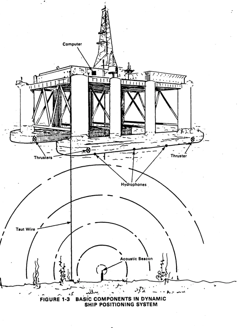
1.3 BASIC COMPONENTS

The basic components in a DP system are illustrated in Figure 1-3. Several types of position measurement systems can be used including taut wire [1], short range radio reference, and sonar systems. These measurements can be pooled and this gives rise to a combination of measurement problems. The heading measurement is given by a gyro­

compass. Communication satellites are increasingly being used to provide a position fix and this enables vessels to be moved to a reference position in just a few minutes. The control force is generated from thrusters.

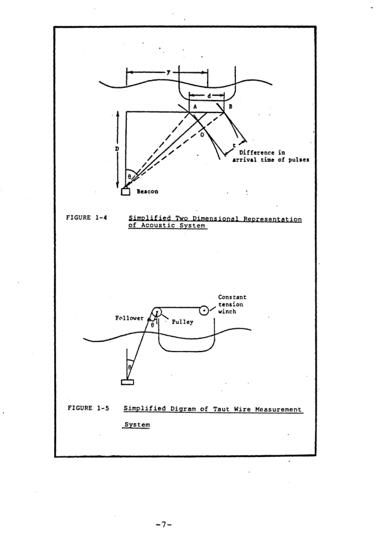
1.3.1 Sonar Measurement System (Figure 1-4)

In the sonar measurement system, an interrogator on board the vessel transmits a sound pu e towards a transponder

which is placed on the seabed or mounted on an object. Upon receipt of a correctly pulsed/coded signal, the transponder transmits a reply. A split beam transducer then performs a highly accurate phase measurement of the received signal and the computer converts the phase angle to the geometric angle of the transponder. At the same time, the accurate range to the transponder is measured, which enables this system to determine the water depth.

-5-Computer

Thruster Thrusters

Hydrophones

Taut Wire

Acoustic Beacon

ci •* • v

Difference in arrival time of pulses

Beacon

FIGURE 1-4 Simplified Two D i m e n s ional Representation of Acoustic System

Constant tension

Follower _{■ Pulley}

FIGURE 1-5 Simplified Digram of Taut Wire Measurement

System

-0/5/mcl704/14

There are many types of acoustic position measurement systems but the GEC/Marconi system was a single beacon on the seabed with a multi-head transponder on a pod beneath the vessel. The signals can be upset by gas bubbles from divers or from the ocean bottom. However, vessels often use more than one position reference system including taut wire,

rig mounted radio beacons and satellite fixes.

1.3.2 Taut Wire Measurement System (Figure 1-5)

The taut wire system is a well established and reliable method of determining the horizontal position of a vessel

relative to a fixed point on the seabed. The required sea­ bed reference point is marked by a sinker weight lowered on a steel wire rope from the vessel. To sense the location of the vessel relative to the sinker weight, the rope is main­ tained under constant tension and the angle of rope from the vertical is measured in two orthogonal axes. The horizontal displacement of the vessel from the seabed reference point is the tangent of these angles multiplied by the water

depth.

1.3.3 Radio Measurement System (Figure 1-6)

Artamis mobile station with calculator and plotter.

REFERENCE DIRECTION

,MOULT*

Artamis tlx station.

FIGURE 1-6 Artemis Range and Bearing Radio Position

0/5/mcl704/15

systems. These systems are used extensively for navigation and survey purposes. However, their position accuracy is not suitable for dynamic positioning. These measurement systems are suitable for applications such as mining and pipelaying. Nevertheless, the short range radio position reference system has a potential for future development. Its operating range is 50 Km with accuracy from 2 m to 20 m at a frequency of 3000 MHz. Basically, it has three modes:

(a) circular,

(b) range/bearing, (c) hyperbolic.

GEC adopts the Artemis range/bearing system (Figure 1-6). The artemis measuring system has the following advantages:

(a) The fixed station equipment is portable and can be set up in approximately half an hour.

(b) One fixed station is sufficient for position fixing of a vessel within line of sight.

(c) The angular accuracy is independent on azimuth. (d) A very low radiated power.

0/5/mcl704/16

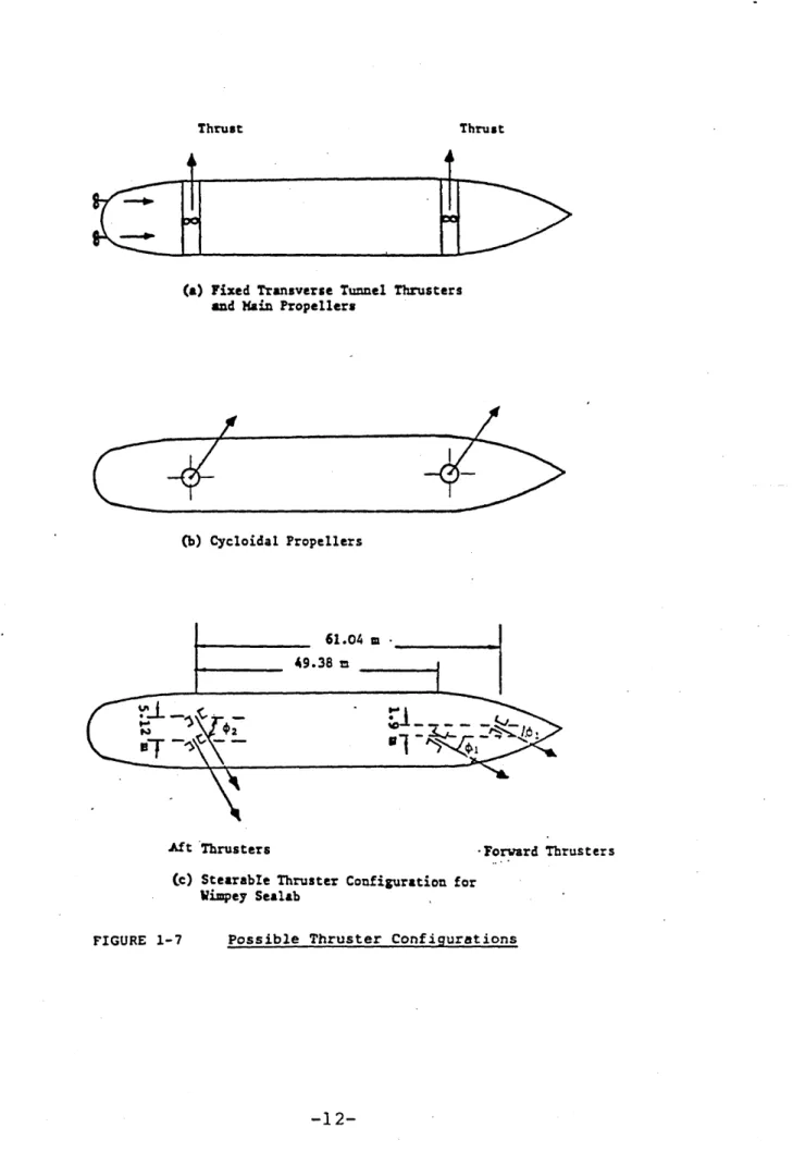
1.3.4 Thrusters

The thruster devices for positioning the vessel can take several forms (Figure 1-7) but the ship model used in the following analysis is based upon Wimpey Sealab which has retractable ac motor driven thrusters with variable pitch propellers. The vessel has two rotatable bow and two

rotatable stern thrusters, capable of 360 degrees rotation and each rated at 12.5 tonnes. The detailed model of the thruster will be discussed in the next chapter.

1.3.5 Wind Speed/Direction Measurement System

The wind force is normally regarded as an environmental disturbance. However, this force can be used in the feed forward loop, which has been shown to improve the control responses significantly. Wind speed and direction are measured by different sensors. However, a package unit

consisting of the two sensors is available, which simplifies the installation and ensures these two parameters are

measured at the same location.

The most commonly used wind speed sensor employs a propeller to drive a small dc voltage generator. The voltage gener­ ated is approximately directly proportional to the speed of

-11-Thrust Thrust

90

(a) Fixed Transverse Tunnel Thrusters and Kain Propellers

(b) Cycloidal Propellers

61.04 m •

•Aft Thrusters

Cc) Stearable Thruster Configuration for Vixspey Sealab

■Forward Thrusters

0/5/mcl704/17

the wind. The output voltage can be calibrated as the measurement of the wind speed.

The wind direction sensor consists of a vane which rotates to track the direction of flow of the wind. Attached to the vane is an angle measuring device which exerts minimum drag on the vane. Commonly used wind sensors are linear

potentiometer and synchro transmitters. The latter has the advantages over the former of avoiding discontinuity and wearing of the components.

-13-0/5/mcl704/18

CHAPTER TWO

DYNAMIC MODELLING OF VESSEL MOTIONS

2.1 THE MOTIONS OF VESSELS

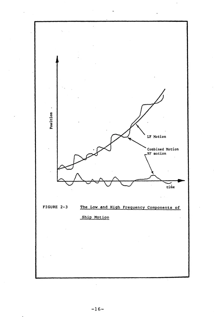
The environmental forces acting on a vessel induce motions in six degrees of freedom (shown in Figure 2-1). In a dynamic positioning system, only vessel motions in the

horizontal plane (surge, sway and yaw) are controlled. All the motions will be referred to the body axes of the vessel (shown in Figure 2-2). The assumption will be made that the low and high frequency vessel motions (Figure 2-3) can be determined separately and that the total motion is the sum of each of them. This is the usual assumption made by a marine engineer because the analysis is simplified and the

low frequency motions can be predicted with more accuracy than the high frequency motions.

The low frequency motions are mainly due to thruster, current, wind and second order wave forces. These are

normally less than 0.25 radians per second. The last three forces can cause the vessel to drift from its station,

surge x

roll $

C.G svay y

pitch 0

\J yav t{/

heave z

FIGURE 2-1 The Motions of Vessel on Sea.

X -"

earth axes

surge x

FIGURE 2-2 Earth and Body Axes Systems

-15-eo o cu

LF Motion

Combined Motion ,HF motion

time

FIGURE 2-3 The Low and High Frequency Components of

0/5/mcl704/19

The first order high frequency wave induced motions are normally oscillating between 0.3 to 1.6 radians per second. These motions are not controlled because the existing

thrusters cannot counteract them effectively. Any attempt will cause unnecessary wear and use extra energy.

In practice, most applications can allow such errors in the controlled variables, particularly in calm sea conditions.

2.2 THE NON-LINEAR LOW FREQUENCY SHIP MODEL

The forces which produce the low frequency (LF) motions are listed as follows:

(a) Forces generated by the thrusters and propellers.

(b) Wind forces. The horizontal wind speed can be resolved into a component in the average wind direction and a component perpendicular to this direction with zero mean. Both components can be modelled by a random variable with a Gaussian probability distribution. (c) Wave induced drift forces. These second order wave

forces are relatively steady and are assumed to be unaffected by the current forces which are almost

constant.

(d) Hydrodynamic forces, caused by the vessel's motion relative to the water. These forces are due to

-17-0/5/mcl704/20

mass, wave generation, viscous drag and hydrostatic buoyancy.

The non-linear differential equation relating surge, sway and yaw velocities are represented by the following form

[2,3].

(M-X^)u - (M-Y^)rv = XA + XH (u,v,r)

(M-Y^)v + (M-Xu )ru = YA +.YH (u,v,r) (2.1)

(I^zz “ ^£-)r = Na + NH (u ,v ,r )

where

u: surge velocity

v: sway velocity

r: yaw velocity

X : applied surge direction force due to

the thruster and the environment

Ya : applied sway direction force due to

the thruster and the environment

Na : applied turning moment on the vessel

xH'yH/nH : the hydrodynamic forces and moment

due to relative motion between the vessel and water

Xu ,Y^,N£-: add masses and add inertia which depend on the

0/5/mcl704/21

M: mass of vessel

I2Z: radius of gyration

The coefficients of this non-linear model are to be

determined by a combination of theoretical analysis and model tank tests [4], The thruster force f is a function of

the control signal in the linearized model. The thruster dynamics will be discussed later in this section.

2.3 THE LINEARIZED LOW FREQUENCY SHIP MODEL

The linear LF ship model is determined by linearizing the non-linear model about an operating point of assumed current flow. This model and the linearized thruster model will be used in system design. The linear model has very little interaction between surge motion and sway/yaw motions, thence, surge motion control will be treated as a separate entity.

The state space equation for the surge motion is:

- - - — — - - —

. su su su SU nSU

X1 all 0 X1

p

. su

x2 1 0 x2su + 0 (2.2)

-19-0/5/mcl704/22

+ psu Uisu ._{+ > '}

0 0

f

su

The sway and yaw state space equations are:

X1 x2 x3 x4

all 0 a13 0

1 0 0 0

a31 0 a33 0

0 0 1 0

xl _{> 1} 0

x 2 0 0

x3 + 0 _h

x4 0 0

/3l 0 0 0 0 02 0 0

u)i u)2 h 0 0 0 0 ₀₂ 0 0 7J2 Fl Tl where

su , ..

xi : surge velocity

su ...

X2 : surge position

xi: sway velocity

X2: sway position

X3: yaw angular velocity

X 4 : yaw angle

Fsu: achieved thrust in surge direction

Fi: achieved thrust in sway direction

T^: achieved torque in yaw direction

o^u : random force applied to surge direction c*>i: random force applied to sway direction 0>2: random torque applied to yaw direction

0/5/mcl704/23

The disturbances such as wave drift and current forces are considered to produce an unknown mean value on the random

forces. The parameters in the system matrices resulted from linearization.

2.4 THRUSTER ALLOCATION LOGIC

The function of the thruster allocation logic is to operate on the demands for thrust in the three axes from the state feedback control to:

(a) Set the thrusters so that the demands are met as closely as possible.

(b) Produce an achieved thrust command signal in each of the three axes for the input into the estimator.

The inputs to the thruster logic are:

(a) Fmax: maximum achieved thrust of the thrusters.

(k) distances of the thrusters from the vessel's

center of gravity.

(c) XU ,YU ,NU : the demanded forces and moment from the state feedback controller.

-21-0/5/mcl704/24

The outputs are:

(a) F].,F2: achieved thrust command signals of the

thrusters.

(b) <f>i, <p2' the angle setting of the thrusters. (c) Xp,Yp,Np: the achieved forces and moment in

surge, sway and yaw direction.

The configuration is illustrated in Figure 2-4.

The thruster allocation logic is a static optimization problem, where minimum fuel consumption is the target. It will be treated as a separate entity and will not be

included in the Kalman filter model. The Kalman filter and the state feedback controller will be concerned only with the thrust in surge and sway axes and moment about the yaw axis. The detailed thruster algorithm is very complicated and it will not be discussed in this report.

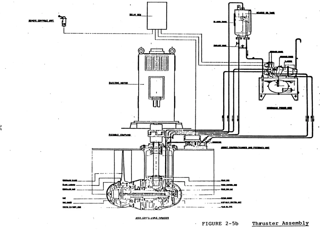
2.5 THE NON-LINEAR THRUSTER MODEL [4]

The thruster devices for dynamic positioning of a vessel can take several forms, but the ship model used in the following is based upon Wimpey Sealab which has retractable ac motor driven thrusters with variable pitch propellers

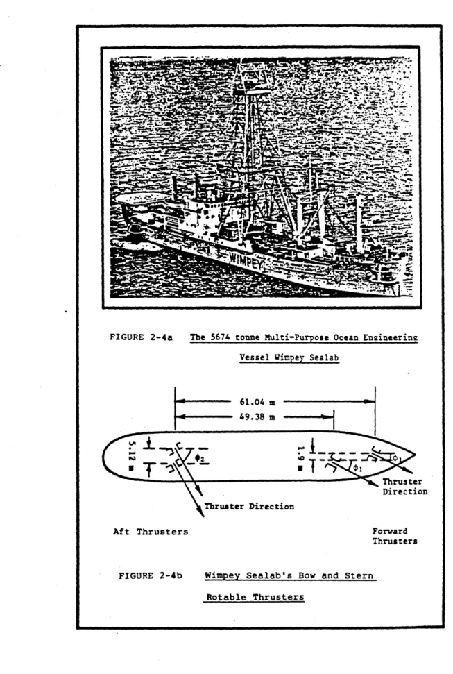
FIGURE 2-4a The 5674 tonne Multi-Purpose Ocean Engineering

Vessel Wiapey Sealab

61.04 a 49.38 a

vo —.3XJLZ. ■ f

Thruster Direction Thruster Direction

Aft Thrusters Forward

Thrusters

FIGURE 2-4b W i m p e y Sealab's Bow and Stern

Rotable Thrusters

-23-ft 8 -23-ft -23-ft -23-ft * « « -23-ft « -23-ft

in ro

M

Is* >2

IliJi

► • • I t s

BHBuacaujsx

-2

0/5/mcl704/25

rotatable stern thrusters which can rotate 360 degrees and are each rated at 12.5 tonnes. The non-linear model is shown in Figure 2-6. The detailed thruster model is very complicated [10]. However, this simplified model is

adequate for the purpose of control analysis.

The input servo is of bang-bang type. It has an electrical input circuit which compares a reference voltage against an electrical feedback from potentiometers measuring the moment of the ram. The error signal is applied to comparators

which switch the forward or reverse solenoid valves when the error exceeds a predetermined deadband. This deadband is set to stop the servo from hunting.

The spring box between the input servo and output servo restricts the force exerted on the mechanical linkage between the two servos. This is approximated by a saturation non-linearity.

The non-linearity between the spring box and the input to the main servo is not great for the angular movement is small, thence, it is assumed to be linear.

Co mp en sa to r In pu t se rv o

- 2

i

!

il

<8*-CO CD

rr\ vo

_{• p.}

o

I

t

£

N

CD

_CO

_•

o

CD <\ o

CD•

K-•i

o

ii

1 °

_{► H}

U "H P , P .

X

8

N

T-

•

c—

CO•

o

0) •o₀ JE U 0) 4J₁₀ 3 u X &■* u 10 0)

c

1c

o •oQl>

0)

'H

C\l

C\J

o

-0/5/mc1704/26

switch is passed through an integrator and then a saturation non-linearity. The scale factor inserted in the feedback loop is the inverse of this saturation element. In

practice, the output servo is faster than the input servo, so the steady state loop gain should be greater than that in the input servo. The ram should move to 100 percent in less than 5 seconds. The actual non-linearities in the forward path and feedback path are not known but can be seen from the experimental curves, that, they can be either

compensated or neglected if small.

The most severe non-linearity is at the thrust and pitch relationship:

Thrust = (pitch)111 m = 1.76 (2.4)

It is usual to compensate for this non-linearity using an input compensator of the form:

1_ m

SQ = (Si) (2.5)

The parameters at the input and the output of the thruster model are scaling factors which normalize the model with

0/5/mcl704/27

2.6 THE LINEAR THRUSTER MODELS

2.6.1 First Order Approximation

The linear model is a fundamental requirement for linear Kalman filter and state feedback controller design. The order of the linear model is quite critical to the

computing load and accuracy of the model. A first order lag approximation was proposed by Grimble et. al. [5,6,7]. For the ith thruster, it takes the following form:

xi(t) = -bixi(t) + biui(t) (2.6)

where 1 / 5 is the time constant of the thruster and u^ is the i

control signal from the controller. xi(t) is the achieved thrust.

The parameter bi is the input amplitude and is frequency dependent. The usual modelling technique is first to estimate the current and wind forces as well as the operating frequency range. The time constant is then

estimated by frequency response or step response techniques.

2.6.2 Second Order Lag Approximation

Fung et. al. [8] proposed a second order linear model to the non-linear thruster. It is well known that a high order

-29-0/5/mcl704/28

linear model is usually a better approximation to the

non-linear model. On the other hand, it will increase the computing load. Then, the choice of the order should depend on these two factors: complexity and accuracy. In the

dynamic ship positioning system, a second order linear

thruster model would only place a small increase on the computing load when using a fixed Kalman filtering scheme yet it has been shown that it gives better estimation [9] of the states and improve the robustness of the control

system. The state equation of the second order linear model has the following form:

xi(t) _{-bi -b2} xifc(t ) 1 _{cr ro ..} I

X2( t) = 1 0 X2 (t ) + 0

Where xi (t) is the thrust rate, x|(t) i u( t )

(2.7)

thrust, u(t) is the demand control signal, bi and b2 are the linearized parameters. The method to estimate these parameters is the same as that described in Section 2.6.1.

2.7 THE DYNAMIC MODEL OF WIMPEY SEALAB

Wimpey Sealab is a dynamically positioned vessel for a variety of operational duties in off-shore exploration

0/5/mcl704/29

overall length of 99.11 metres, a beam of 15.24 metres and a displacement of 5674 tonnes. The position is automatically controlled by a computer which controls the operation of four 1,000 HP (746 Kw) retractable thrusters, each fitted with variable pitch propellers [10] and capable of 360° rotation. The vessel is equipped with acoustic and taut wire position reference systems. Wimpey Sealab also has a satellite navigation system which enables the vessel to position itself accurately at predetermined locations and has an integrated Doppler Sonar System for traversing predetermined paths to very high orders of accuracy• The specifications of the vessel for control system analysis are listed in Appendix B.

GEC Electrical Projects Ltd. is responsible for the control system design.

Dynamic positioning for Wimpey Sealab is required in water depths between 30 and 300 metres. The ship must be held within a circle of 7 metres radius (or 3% of water depth, whichever is the greater) in a steady wind of up to

12.87 m/sec. with waves of significant height, 3.54 metres and significant length 91.44 metres and with a steady sea current up to 1.54 m/sec. Under the above conditions, but with the wind gusting up to 20.50 m/sec, the ship position

-31-0/5/mcl704/30

must be held within a circle of 11 metres radius. Ship heading is allowed to vary.

2.7.1 The Low Frequency Model

The normalized non-linear differential equation reference of the vessel are [1 1]:

1.044 u = XA + 0.092 v^ - 0.138 uU + 1.84 rv

1.840 v = YA - 2.580 vU - 1.840 v3/U + 0.068 r|rJ-rU 0.1021 r = NA - 0.764 uv + 0.258 vU - 0.162 r|r|(2.8)

The variables are defined in equation 2.1. U is the vector sum of u and v.

The linear LF model, under zero current flow, is:

1.044 u = XA - 0.0159 u

1.840 v = Ya - 0.1004 v + 0.002981 r (2.9)

0.10221r = Na - 0.007101 r + 0.005859v

0/5/mcl704/31

case. It can be solved easily once the control system for the multivariable case is established.

The linearized state equation of the ship model, together with the thrusters, is of the following form:

A| (fc) = A* *1 + Hjt(t) + (t) + (t)

y ^ (t ) = Cj x ^ (t ) (2.10)

Where U j ( t ) £ is the control input to the thrusters, ^ (t )

£ r2 is a white noise sequence representing the random forces applied to the vessel and R^ is the wind force

disturbances. Other disturbance forces, such as wave drift and current forces cannot be measured but can be considered to produce an unknown mean value on the signal o^(t), the vector y^(t)6 R^ represents the position outputs: sway and yaw.

In Section 2.6, the linear thruster model can be either

first order or second order, thence state vector and

the system matrices are different in each case. Model A and Model B given below represent two different models for

control system design. Let the system matrices be partitioned into the following forms:

-33-0/5/mcl704/32

Ai = 0

11 A l2 A(2 2

1

O

J

' D n

03

r— It _{y \} cf- it ₁

o

1

II 1 M

1 c 11 Lt 0 ii r 0 (2.11)

xt (t) = x^ 1 (t )

x-H(t)6R^ * x2 1(t) is dependent on the model used. Matrices A.ll,

_X

_i

_l

_{l i}

_—g

both models. Matrices A^22 and q21 are dependent on the

thruster model selected. All linearized equations have been time scaled with 3.104 as a time normalization factor.

Xj (t)

11

12

xi sway velocity

x 2 sway position

x3 yaw angular velocity (2

x4 yaw angle

-0

.

1.0 0 0 0

0

.

0 0 1 . 0 0

0.5435 0 _{D/U =} 0.5435 0

0 0 0 0

0 -1.6340 0 9.785

0/5/mcl704/33 11 _0.384 0 0 0 0 0 6.92 0

c.n = 0 1 0 0

0 0 0 1

(2.13)

There are two linear ship models to be used in the

simulation analysis. The difference between these models is in the thruster subsystems only.

Model A

x5 x6

a22=

Rt

thruster one thruster two

-1.55 0

0 -1.55 b21 =

1. 55 0 0 1.55 (2.14) (2.15)

In this model, the time constants of the thrusters are all 2 seconds (0.644 per unit).

Model B

x5

x6

x7 x8

thrust rate of thruster one thrust of thruster one

thrust rate of thruster two thrust of thruster two

(2.16)

-35-0/5/mcl704/34

The time constants obtained by fitting the best second order linear model to the non-linear thrusters using frequency tests and Bode diagrams are:

TABLE 2-1

PEAK SINE WAVE INPUT TIME CONSTANTS (PER UNIT)

1*1

t

0.0002 0.3981 0.3055

0.0005 0.7244 0.4266

0.001 1.059 0.6918

0. 0022 1/585 0. 861

Note that one unit is equivalent to input amplitude of 0.0022. The time constants used in the linear model were taken as T^ = 1.059 and T2 = 0.6918 seconds which

0/5/mcl704/35

A? * -2.3895 -1.3646

1.0 0

0 0

0 0

0 0 -2.3895 -1.3646

0 0 1.0 0

B£21= 1. 3646 0

0 0

0

1.3646 (2.17)

0 0

In the full LF model, two zero columns should be added to

2.7.2 The Noise Covariances Specifications

The process noise in the dynamic positioning problem can be partitioned into two parts: high frequency model and low frequency model. Let 0^ and 0^ be their covariance matrices respectively. Oh is assumed to be unity. The Qj covariance matrix is dependent on the mean wind force level. In Wimpey Sealab tests, the following values have been taken:

= sway per unit force covariance

= (0.00228)2 = 5.2 x 1CT6 C: 4 x 10“ 6

Qj2 = yaw per unit torque covariance

= (0.00031)2 = 9.6 x 10" 8 £: 9 x 10“ 8

the RHS of matrix A^2 to complete a square matrix A|

-37-0/5/incl704/36

Thence the process noise covariance matrix for the total system is:

Of =

4xl0“6 _o i_{; 0 0}

0 9xicr8 !

1 0 0

0 0 1₁ 1 0

0 0 1 0 1

(2.18)

The position measurement error is assumed to be 0.333 metre. In the normalized unit, it is 0.0033.

Therefore, the noise variance for sway motion is RjgicrlO” ^* The yaw standard deviation is assumed to be 0.2 degrees, so that R£2 ^ 1 * 2 2 x 10“5. Thence, the measurement noise

covariance matrix is:

10“5 0

1 . 2 2 x 1 0 “ 5

(2.19)

2.8 HIGH FREQUENCY MODEL

The high frequency motions of the vessel are in sympathy with the wave frequencies, and are assumed to be linearly related to the wave forces. The spectrum of the high frequency vessel motion is obtained from a standard sea

0/5/mcl704/37

sea spectrum alone which means the wave motions are not attenuated by the vessel dynamics.

Several sea wave spectra [12] have been proposed. A

commonly used one is the Pierson-Moskowitz model [13] which is expressed by:

where qo is the angular frequency in radians per second.

A = 4. 894 , B =3. 1094/(h^) 2. The term h^ is defined as the significant wave height in metres. By finding the stationary point for Sn (*u), the resonant frequency of the spectrum is found to be:

The wave spectra of several sea conditions (identified by Beaufort Numbers) are shown in Figure 2-7.

There are three types of models used in state estimation

using Kalman filter.

2.8.1 Rational Proper Transfer Function Model

Kostecki [14] suggested the sea spectrum can be approximated by a rational proper transfer function presented by:

(2.20)

= (4B/5 )1/4 (2.21)

-39-.5

0E

+0

2

•H

u_

(N

0/5/mcl704/38

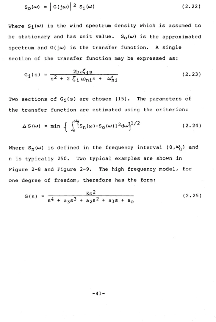
S0(o>) = | G( ju>)

J

Where Si(^) is the wind spectrum density which is assumed to be stationary and has unit value. S0 (u>) is the approximated spectrum and G(joj) is the transfer function. A single

section of the transfer function may be expressed as:

2 b i £ -js

Gi(s) ---

1

s + 2 tOnis + ^ni

Two sections of Gi(s) are chosen [15]. The parameters of the transfer function are estimated using the criterion:

A S (to) = min I y 1 s n (u))-s0 (w)]2d^ 1 / 2 (2.24)

Where Sn (u>) is defined in the frequency interval (0,^g) and n is typically 250. Two typical examples are shown in

XT

CO ₀₀

o

CO O

o

co O

o

_o

_o

r\j

o

o

_o

- BO

co *c o o

CM

-S

o

C\J

00

o

00

o

60

'O

o

o>

o

o

o

in

o

o

•

-S3

60

*0

o

-4

0/5/mcl704/39

In state space form:

ih<t> = Fhih(t) + Gh^(t)

Yh(t) = Hhxh (t)

(

.

)

Where

*h

(t) 6 R12, ^h(t)

e

R3

F®U _h 0 0 G®U _h 0 0

Fh - 0 F? h 0 - S = 0 Gh 0

0 0 _h 0 0 _h

Hh = n?uh

o o

0 Hh 0 (2.27)

0/5/mcl704/40

0 1 0 0 0

0 0 1 0 _{Gh =} 0

0 0 0 1 ₀

_-fo -fs2 - f s3

..

.

1

O)

i

[0 0 hs₃ 0]

2.8.2 Auto-Regressive Moving Average (ARMA) Model

This model was first used in the DP Kalman filter estimation by Fung and Grimble [16]. It is assumed that the high

frequency disturbance can be epresented by the following multivariable ARMA model:

Ahfz”1 ) = Chfz"1 ) |_h(t) (2.29)

which is assumed to be asymptotically stable and yh(t)£R^

and ih (t) 6 R^, Here, §_h(t) represents an independent zero mean random vector which is uncorrelated with the low

frequency disturbances and the measurement noise. The covariance matrix of £h(t) *-s denoted by ^ h *

polynomial matrices A ^ z ”1 ) and C ^ z ”1 ) are assumed to be

square and of the form:

-45-0/5/mcl704/41

= I3 + Aiz”l+ +Anaz_na Ch (z“i) = Ciz” 1 + C2Z-2+.,+Cncz-nc

(2.30) (2.31)

where z” l is the backward shift operator. The matrix Ah(z“l) is assumed to be regular (that is Ana is non- singular). The zeros of det (An (x)) and det (Cft(X)) are assumed to be strictly outside the unit circle. The order of the polynomial matrices are known but the coefficients

constant or slow varying unknowns since in practice, the wave spectrum varies slowly with weather conditions. It is also assumed that the disturbances in each observed channel

diagonal form.

2.8.3 Harmonic Oscillation Model

The harmonic oscillation model for high frequency motions of a vessel for dynamic control system was discussed in

[17,18], The surge, sway and yaw motions are modelled by three separate harmonic oscillators. Each oscillator has a variable frequency, a white noise input representing

the modelling error and unpredictable wave noise. The state space representation of HF motions becomes:

na' ...nc , are treated as

0/5/mcl704/42

Xh(t) = Fh xh (t) + Gft £_h (t )

yh(t) = Hh xj^t) (2.32)

where:

Xhl(t)

Xh2<t)

HF

Xh3(t> HF

xh (l:)

xh4(t)

u?2

xh5(t)

xh6(t)

^3 HF

Fhl 0 0

Fh = 0 _Fh2 0

0 0 _Fh3

Hh i 0 0

Hh = 0 _Hh2 0

0 0 _«h3

0 1 0

ri «. up" n

Fhi - —It/* i u u

0 0 0

i = 1, 2, 3

Gh =

hi

®hl 0 0

0 _^h2 0

0 0 _°h3

-47-0/5/mcl704/43

x ^ t ) 6 is the state variable Jh(t)6 R^ is the high

frequency motions, 6 R^ is the process white noise

sequence.

2.8.4 Simulation of High Frequency Motions

Method 1

The first order wave induced HF motions can be simulated using the following expression [19] (in one direction with

unit in metre):

M

yh(t). = 2. y0sin(Ct>it+^i) (2.35)

i = l

where ©i are random numbers lying in (0, 27f), yQ and are selected to approximate the Pierson-Moskowitz wave

spectrum. M is the number of equal parts (in terms of

energy) into which the wave spectrum is divided. A typical

value of M is 20.

0/5/mcl704/44

= 0 -6990-52-5 x I n (

A

pad/sBC- (2.36)

y0 = h1/3 (M/2 )“1/2 naetr&S (2.37)

Other terms such as wind speed and Beaufort number are also used to characterize the sea conditions.

Method 2

This method uses the rational proper transfer function of HF motions described in Section 2.8.1 to simulate sea waves.

For each weather condition, the parameters of the model are estimated using least squares technique. The state space representation of the model is used to generate the HF motions. Since the model is assumed to be linear, a

discrete model is more appropriate for updating the states. A set of values for some typical weather conditions are given in Appendix A.

2.9 THE LINEAR STATE SPACE EQUATIONS FOR SHIP MOTIONS

The state equations for the low and high frequency models of the ship can be combined into the form:

-49-0/5/mcl704/45

i,(t>

Xh(t)

AX 0 0 Fh

£ i (t) +

x.h(t) 0

ju x (t ) +

i

&

i

rj_ (t) + i d* o r

0 _{_° G h _}

The position of the vessel is given and high frequency motions:

t )

o^h (t ) (2.38)

£ ( t ) = £ j ( t ) + £ h ( t ) (2.39)

The position measurement Z(t) sway and yaw is therefore:

zx (t) = [Cjj Hh ] XI -4 4-1 1 ~

1

+ v(t)

z2(t) _{2£h (t )} (2.40

= ) + Yh ( ) + X ( )

where v(t) = [v^ V2lT is a white noise signal representing measurement system noise. The above equations can be

written more concisely as:

x(t) = Ax(t) + Bu(t) + E^(t) + Dcu(t) z(t) = Cx(t) + v(t)

0/5/mcl704/46

where u_ (t ) includes the control signals, ^(t) includes the measurable disturbances inputs, ojjt) represents the white

process noise input and v(t) represents the white measurement noise signal. These equations are in the standard form associated with the Kalman filtering and optimal stochastic control problem.

-51-0/5/mcl704/47

CHAPTER THREE

KALMAN FILTERING PROBLEM OF DYNAMIC SHIP POSITIONING SYSTEMS

3.1 THE ESTIMATION STRUCTURE

The stochastic model of the vessel is defined by the state equation in Section 2.9, and now the estimation problem can be considered. Recall that for control purposes, it is not simply the total position y_(t) of the vessel that is to be estimated, but rather the low frequency component X|(t). That is, the position control problem must only respond to the low frequency position error signal. The estimator is

A

therefore required to provide an estimate y^(t). If a state feedback controller is to be implemented, the states in the low frequency model must be estimated. If a stochastic

model of a system is formed the Kalman filtering solution is quite standard nowadays [20, 21]. The Kalman filter

includes a model of the total system and can therefore

provide the high and low frequency motion estimates. The DP Kalman filter structure is shown in Figure 3-1 and is

Ml

*1

U I

n

•( BJ

-53-0/5/mcl704/48

>c(t) = Ax(t) + K(t) Iz^(t) - Cx(t)] + Bu (t ) + E_J(t)

(3.1)

£(t) = Cx(t) (3.2)

The Kalman gain matrix K(t) can be partitioned into low and high frequency matrices as follows:

This matrix can be calculated for given noise covariance matrices by using standard results (Appendix C). The measurement noise covariance can be defined relatively accurately from the knowledge of the position measurement system and using manufacturers data. The process noise covariance matrix is less well defined (Section 2.7).

In practice, the process noise of the LF model and the

measurement noise can be assumed stationary. The LF linear model with respect to a current force can be assumed

constant. However, the HF model is based upon sea spectra which vary with sea conditions. The variations may be very slow but nevertheless, the Kalman gain Kj^(t) and the

parameters in the model vary with the weather conditions. To implement an optimal Kalman filter, the Kalman gains and the parameters in the models need updating, that means the

K(t) K| (t)