Normality tests for dependent data: large sample and bootstrap approaches

BIROn - Birkbeck Institutional Research Online

Psaradakis, Zacharias and Vávra, M. (2018) Normality tests for dependent

data: large-sample and bootstrap approaches. Communications in Statistics

- Simulation and Computation , ISSN 0361-0918. (In Press)

Downloaded from:

Usage Guidelines:

Please refer to usage guidelines at or alternatively

Normality Tests for Dependent Data:

Large-Sample and Bootstrap Approaches

∗

Zacharias Psaradakis

Department of Economics, Mathematics and Statistics

Birkbeck, University of London

E-mail:

z.psaradakis@bbk.ac.uk

Mari´

an V´

avra

Research Department, National Bank of Slovakia

Birkbeck Centre for Applied Macroeconomics

E-mail:

marian.vavra@nbs.sk

This version: May 31, 2018

Abstract

The paper considers the problem of testing for normality of the one-dimensional marginal distribution of a strictly stationary and weakly dependent stochastic process. The possibility of using an autoregressive sieve bootstrap procedure to obtain critical values and P-values for normality tests is explored. The small-sample properties of a variety of tests are investigated in an extensive set of Monte Carlo experiments. The bootstrap version of the classical skewness–kurtosis test is shown to have the best overall performance in small samples.

Key words: Autoregressive sieve bootstrap; Normality test; Weak dependence.

∗_{We wish to thank an anonymous referee for helpful comments. We are also grateful to Antonio}

1

Introduction

The problem of testing whether a sample of observations comes from a Gaussian dis-tribution has attracted considerable attention over the years. This is not perhaps surprising in view of the fact that normality is a common maintained assumption in a wide variety of statistical procedures, including estimation, inference, and forecasting procedures. In the context of model building, a test for normality is often a useful diagnostic for assessing whether a particular type of stochastic model may provide an appropriate characterization of the data (for instance, non-linear models are unlikely to be an adequate approximation to a time series having a Gaussian one-dimensional marginal distribution). Normality tests may also be useful in evaluating the validity of different hypotheses and models to the extent that the latter rely on or imply Gaussian-ity, as is the case, for example, with some option pricing, asset pricing, and dynamic stochastic general equilibrium models found in the economics and finance literature. Other examples where normality or otherwise of the marginal distribution is of inter-est, include value-at-risk calculations (e.g.,Cotter(2007)), and copula-based modelling for multivariate time series with the marginal distribution and the copula function being specified separately. Kilian and Demiroglu (2000) and Bontemps and Meddahi (2005) give further examples where testing for normality is of interest.

Although most of the literature on tests for normality has focused on the case of independent and identically distributed (i.i.d.) observations (see Thode (2002) for an extensive review), a number of tests which are valid for dependent data have also been proposed. These include tests based on empirical standardized cumulants (Lobato and Velasco (2004), Bai and Ng (2005)), moment conditions of various types (e.g., Epps

(1987), Moulines and Choukri (1996), Bontemps and Meddahi (2005)), the bispectral density function (e.g.,Hinich(1982),Nusrat and Harvill(2008),Berg et al.(2010)), and the empirical distribution function (Psaradakis and V´avra (2017)). Unlike normality tests for i.i.d. observations, whose finite-sample behaviour has been extensively studied (see, inter alia,Baringhaus et al.(1989),Rom˜ao et al.(2010), andYap and Sim(2011)), a similar comparison, across a common set of data-generating mechanisms, of tests designed for dependent data is not currently available in the literature.

Our aim in this paper is twofold. First, we wish to investigate the small-sample size and power properties of tests for normality of the one-dimensional marginal distri-bution of a strictly stationary time series. The tests under consideration are some of those mentioned in the previous paragraph, as well as tests that rely on the empirical characteristic function of the data and on order statistics. Second, since in the presence of serial dependence conventional large-sample approximations to the null distributions of some of the test statistics under consideration are inaccurate, unknown, or depend on the correlation structure of the data in complicated ways, we wish to investigate the possibility of using bootstrap resampling to implement tests of normality. More specifically, we consider estimating the null sampling distributions of the test statistics of interest by means of the so-called autoregressive sieve bootstrap, and thus obtain

P-values and/or critical values for normality tests. The bootstrap method is based on the idea of approximating the data-generating mechanism by an autoregressive sieve, that is, a sequence of autoregressive models the order of which increases with the sam-ple size (e.g., Kreiss (1992), B¨uhlmann (1997)). Bootstrap-based normality tests are straightforward to implement and, as our simulation experiments demonstrate, offer significant improvements over asymptotic tests, that is, tests that use critical values from the large-sample null distributions of the relevant test statistics.

examines the small-sample properties of asymptotic and bootstrap-based normality tests by means of Monte Carlo simulations. Section5 summarizes and concludes.

2

Problem and Tests

2.1

Statement of the Problem

Suppose that (X1, X2, . . . , Xn) arenconsecutive observations from a strictly stationary, real-valued, discrete-time stochastic processX ={Xt}∞t=−∞ having mean µX =E(Xt) and varianceσ2

X =E[(Xt−µX)2]>0. It is assumed thatX is weakly dependent, in the sense that its autocovariance sequence decays towards zero sufficiently fast so that the seriesP∞_τ=0Cov(Xt, Xt−τ) converges absolutely (and, consequently,X has a continuous and bounded spectral density). The problem of interest is to test the composite null hypothesis that the one-dimensional marginal distribution ofX is Gaussian, that is,

H0 : (Xt−µX)/σX ∼N(0,1), (1)

where a tilde ‘_∼’ means ‘is distributed as’. The alternative hypothesis is that the distribution ofXt is non-Gaussian.

2.2

Tests Based on Skewness and Kurtosis

Bowman and Shenton(1975) andJarque and Bera(1987) proposed a test for normality based on the empirical standardized third and fourth cumulants, exploiting the fact that for a normal distribution all cumulants of order higher than the second are zero. The test statistic is given by

J B= nµˆ 2 3 6ˆµ3₂ +

n(ˆµ4−3ˆµ22)2

24ˆµ4₂ , (2)

where, for an integer r _> 2, ˆµr = (1/n) Pn

t=1(Xt−X¯)r and ¯X = (1/n) Pn

t=1Xt. For Gaussian i.i.d. data, J B is approximately χ2

2 distributed for large n. Although a test which rejects whenJ B exceeds an appropriate quantile of the χ2

2 distribution is clearly not guaranteed to have correct asymptotic level in the presence of serial dependence, it is arguably the most popular normality test in the literature and is available in many statistical and econometric packages (e.g., EViews, Matlab, Stata). It will, thus, serve as a benchmark for comparisons in our study.

Bai and Ng (2005) developed a related test which allows for weak dependence in the data. The test is based on the statistic

BN = nµˆ 2 3 ˆ

ζ3µˆ32

+ n(ˆµ4−3ˆµ 2 2)2 ˆ

ζ4µˆ42

, (3)

where ˆζ3 and ˆζ4 are consistent estimators of the asymptotic variance of √

nµˆ−₂3/2µˆ3 and √

the triangular Bartlett kernel and a data-dependent bandwidth, selected according to the method of Andrews(1991), are used.

An alternative test, also based on skewness and kurtosis, was proposed by Lobato and Velasco(2004). The test statistic is defined as

LV = nµˆ 2 3 6 ˆG3

+n(ˆµ4−3ˆµ 2 2)2 24 ˆG4

, (4)

where ˆGr = Pn−1

τ=1−nγˆ r

τ for r = 3,4 and ˆγτ = (1/n) Pn

t=|τ|+1(Xt−X¯)(Xt−|τ|−X¯) for

τ = 0,±1, . . . ,±(n−1). An advantage of the test based on LV is that the estimators of the asymptotic variance of √nµˆ3 and

√

n(ˆµ4−3ˆµ22) used do not involve any kernel smoothing or truncation (in contrast to the estimators ˆζ3 and ˆζ4 used in the case of

BN). If X is a Gaussian process, BN and LV are approximately χ2₂ distributed for largen.

2.3

Test Based on Moment Conditions

Bontemps and Meddahi(2005) proposed a test based on moment conditions implied by the characterization of the normal distribution given inStein(1972). The test is based on the statistic

BM = √1

n n X t=1 ˆ gt ! ˆ

Σ−1 √1

n

n X

t=1

ˆ g_t0

!

, (5)

whereˆgt= (h3(Zt), . . . , h`(Zt)) for some integer`>3,Zt={nµˆ2/(n−1)}−1/2(Xt−X¯), and Σˆ is a consistent estimator of the long-run covariance matrix of {ˆgt}. Here, hm(·) stands for the normalized Hermite polynomial of degreem, given by

hm(x) = √

m! bm/2c

X

i=0

(−1)i_xm−2i

i!(m−2i)!2i, −∞< x <∞, m = 0,1,2, . . . ,

where bac denotes the largest integer not greater than a. Under H0, BM is approxi-mately χ2

`−2 distributed for largen.

As in the case of the BN statistic, Σˆ is constructed using a Bartlett-kernel esti-mator with a data-dependent bandwidth chosen by the method ofAndrews (1991). In light of the relatively poor small-sample size properties of the test reported inBontemps and Meddahi (2005) for dependent data when Hermite polynomials of degree higher than 4 are used, we set `= 4 in our implementation of the test.

2.4

Tests Based on the Empirical Distribution Function

Psaradakis and V´avra(2017) considered a test based on the Anderson–Darling distance statistic involving the weighted quadratic distance of the empirical distribution function of the data from a Gaussian distribution function. Putting Yt = ˆµ

−1/2

test rejectsH0 for large values of the statistic

AD = n

Z ∞

−∞

{FˆY(y)−Φ(y)}2

Φ(y){1−Φ(y)} dΦ(y)

= −n− 1

n

n X

t=1

(2t−1) [log Φ(Y(t)) + log{1−Φ(Y(n+1−t))}], (6)

where ˆFY is the empirical distribution function of (Y1, . . . , Yn),Y(1) 6· · ·6Y(n) are the order statistics of (Y1, . . . , Yn), and Φ is the standard normal distribution function. In the sequel, we also consider tests which reject H0 for large values of the Cram´er–von Mises statistic

CM =n

Z ∞

−∞

{FˆY(y)−Φ(y)}2dΦ(y) = 1 12n +

n X

t=1

Φ(Y(t))−

2t−1 2n

2

, (7)

or the Kolmogorov–Smirnov statistic

KS = √n sup −∞<y<∞

|FˆY(y)−Φ(y)|

= √n max 16t6n

t

n −Φ(Y(t)),Φ(Y(t))− t−1

n ,0

. (8)

Since the asymptotic null distributions of these statistics have a rather complicated structure in the case of a composite null hypothesis even under i.i.d. conditions (cf.

Durbin (1973), Stephens (1976)), critical values and/or P-values for the tests will be obtained by a suitable bootstrap procedure. Stute et al.(1993), Babu and Rao(2004), andKojadinovic and Yan(2012) also considered bootstrap-based approaches to testing composite hypotheses for i.i.d. data, whilePsaradakis and V´avra(2017) examined the case of linear processes that may exhibit strong, weak, or negative dependence.

2.5

Test Based on the Empirical Characteristic Function

Epps and Pulley (1983) proposed a class of tests based on the weighted quadratic distance of the empirical characteristic function of the data from its pointwise limit under the null hypothesis of normality. Using the density of theN(0,1/µˆ2) distribution as a weight function (cf. Epps and Pulley (1983)), the test rejects H0 for large values of the statistic

EP = n

Z ∞

−∞

|ϕˆY(u)−ϕ(u)|2dΦ(ˆµ 1/2 2 u)

= √n 3+ 1 n n X t=1 n X s=1

exp−1

2(Yt−Ys) 2

−√2 n X

t=1

exp −1 4Y

2 t

(9)

For Gaussian i.i.d. data, EP is asymptotically distributed as a weighted sum of infinitely many independent χ2

1 random variables (Baringhaus and Henze (1988)). To the best of our knowledge, the asymptotic distribution ofEP has not been established in the case of dependent data. We will use a bootstrap procedure to obtain critical and/or

P-values for the test based on EP. We note that, in an i.i.d. context,Jim´enez-Gamero et al. (2003) and Leucht and Neumann(2009) examined bootstrap-based inference for statistics (such as EP, AD, and CM) which may be expressed in the form of, or be approximated by, degenerate V-statistics involving estimated parameters. Leucht

(2012) andLeucht and Neumann(2013) give related results for weakly dependent data.

2.6

Test Based on Order Statistics

Shapiro and Wilk(1965) proposed a test based on the regression of the order statistics of the data on the expected values of order statistics in a sample of the same size from the standard normal distribution. The test rejects H0 for small values of the statistic

SW = 1

nµˆ2 n X

t=1

atX(t) !2

, (10)

where X(1) 6 · · · 6 X(n) are the order statistics of (X1, . . . , Xn) and (a1, . . . , an) are constants such that (n−1)−1/2Pn

t=1atX(t)is best linear unbiased estimator ofσX under (1). For Gaussian i.i.d. data, SW (suitably normalized) is asymptotically distributed as a weighted sum of infinitely many independent and centred χ2₁ random variables (Leslie et al. (1986)).

One difficulty with a test based on SW is that exact or approximate values of the coefficients (a1, . . . , an) are known only under i.i.d. conditions. In the sequel, we use the approximation method suggested byRoyston (1992) to compute these coefficients, while critical values and/or P-values for the test are obtained by means of a bootstrap procedure.

2.7

Test Based on the Bispectrum

Hinich (1982) proposed a test for Gaussianity of a stochastic process based on its normalized bispectrum, exploiting the fact that the latter should be identically zero at all frequency pairs if the process is Gaussian. For some integerk _>1, the test used in the sequel is based on the statistic

H = 2πn

δM2 k X

i=1

|fˆb(ω1,i, ω2,i)|2 ˆ

fs(ω1,i) ˆfs(ω2,i) ˆfs(ω1,i+ω2,i)

, (11)

where ˆfs and ˆfb are kernel-smoothed estimators of the spectral and bispectral density, respectively, ofX, M is a bandwidth parameter associated with ˆfb, δ is a normalizing constant associated with ˆfb, and Ωk = {(ω1,i, ω2,i), i = 1, . . . , k} is a set of frequency pairs contained in Ω ={(ω1, ω2) : 06ω1 6π,06ω2 6min{ω1,2(π−ω1)}} (see Berg

In the sequel, we followBerg et al.(2010) in taking Ωkto be a subset of the grid of points contained in their Fig. 2, as well as in using a trapezoidal flat–top kernel function and a right-pyramidal frustrum-shaped kernel function to construct the estimators ˆfs and ˆfb, respectively. A common bandwidth M =bn1/3c is used for ˆfs and ˆfb, and we set k = bn/10c. We note that Berg et al. (2010) considered using an autoregressive sieve bootstrap approximation to the null distribution ofH as an alternative to theχ2

2k large-sample approximation. Also note that, unlike the testing procedures discussed previously, which assess normality of the one-dimensional marginal distribution of X, the test based onH assesses Gaussianity of the process X (i.e., normality of all finite-dimensional distributions of X).

3

Bootstrap Tests

Some of the normality tests described in Section 2, although asymptotically valid for dependent data, tend to suffer from substantial level distortion in finite samples (e.g., the bispectrum-based test). For some other tests, large-sample approximations to the null distribution of the relevant test statistic may not be straightforward to obtain because of the dependence in the data and the composite null hypothesis (e.g., tests based on the empirical distribution function, the empirical characteristic function, or order statistics). A convenient way of overcoming these difficulties is to use a suitable bootstrap procedure to approximate the sampling distribution of the test statistic of interest under the null hypothesis. In this paper, we propose to use the autoregressive sieve bootstrap to obtain such an approximation and construct bootstrap tests for normality.

The typical assumption underlying the autoregressive sieve bootstrap is that X admits the representation

Xt−µX = ∞ X

j=1

φj(Xt−j−µX) +εt, (12)

where {φj}∞j=1 is an absolutely summable sequence of real numbers and {εt}∞t=−∞ are i.i.d., real-valued, zero-mean random variables with finite, positive variance. The idea is to approximate (12) by a finite-order autoregressive model, the order of which increases simultaneously with the sample size at an appropriate rate, and use this model as the basis of a semi-parametric bootstrap scheme (see, inter alia,Kreiss(1992),Paparoditis

(1996),B¨uhlmann (1997),Choi and Hall (2000), andKreiss et al. (2011)).

Note that, under the additional assumption that the functionφ(z) = 1−P∞_j=1φjzj has no zeros inside or on the complex unit circle, (12) is equivalent to assuming thatX satisfies

Xt =µX + ∞ X

j=0

ψjεt−j, ψ0 = 1, (13)

LettingS =S(X1, . . . , Xn) be a statistic for testing the normality hypothesis (1), the algorithm used to obtain an autoregressive sieve bootstrap approximation to the null distribution of S can be described by the following steps:

S1. For some integer p _>1 (chosen as a function of n so that p increases with n but at a slower rate), compute the pth order least-squares estimate ( ˆφp1, . . . ,φˆpp) of the autoregressive coefficients for X by minimizing

(n−p)−1 n X

t=p+1 (

(Xt−X¯)− p X

j=1

φpj(Xt−j −X¯) )2

. (14)

S2. Given some initial values (X₋∗_p+1, . . . , X₀∗), generate bootstrap pseudo-observations (X₁∗, . . . , X_n∗) via the recursion

X_t∗−X¯ = p X

j=1 ˆ

φpj(Xt∗−j −X¯) + ˆσpε∗t, t= 1,2, . . . , (15)

where ˆσ2

p is the minimum value of (14) and{ε ∗

t}are independent random variables each having the N(0,1) distribution. Define the bootstrap analogue of S by the plug-in rule as S∗ = S(X₁∗, . . . , X_n∗) (i.e., by applying the definition of S to the bootstrap pseudo-data).

S3. Repeat step S2 independently B times to obtain a collection of B replicates (S₁∗, . . . , S_B∗) of S∗. The empirical distribution of (S₁∗, . . . , S_B∗) serves as an ap-proximation to the null distribution of S.

The (simulated) bootstrap P-value for a test that rejects the null hypothesis (1) for large values of S is computed as the proportion of (S₁∗, . . . , S_B∗) greater than the observed value ofS. Hence, for a given nominal levelα (0< α <1), the bootstrap test rejectsH0 if the bootstrap P-value does not exceedα. Equivalently, the bootstrap test of level α rejects H0 if S exceeds the (b(B+ 1)(1−α)c)th largest of (S1∗, . . . , S

∗ B). Some remarks about the bootstrap procedure are in order.

(i) The order p of the autoregressive sieve in step S1 may be selected from a suitable range of values by means of the Akaike information criterion (AIC), so as to minimize log ˆσ_p2+2p/(n−p). Under mild regularity conditions, a data-dependent choice ofpbased on the AIC is asymptotically efficient (see, inter alia,Shibata(1980),Lee and Karagrigoriou (2001), and Poskitt (2007)), and satisfies the growth conditions on the sieve order that are typically required for the asymptotic validity of the sieve bootstrap for a large class of statistics (Psaradakis (2016)).

(iii) By requiringε∗_t in (15) to be normally distributed, the bootstrap pseudo-data {X_t∗}are constructed in a way which reflects the normality hypothesis under test even though X may not satisfy (1). This is important for ensuring that the bootstrap test has reasonable power against departures from H0 (see, e.g., Lehmann and Romano (2005, Sec. 15.6)).

(iv) Some variations of the bootstrap procedure may be obtained by varying the way in which the initial values (X₋∗_p+1, . . . , X₀∗) for the recursion (15) are chosen in step S2. For instance, one possibility is to calculate (X₋∗_p+1, . . . , X₀∗) from the moving-average representation of the fitted autoregressive model for Xt−X¯ (Paparoditis and

Streitberg(1992)). Another possibility is to setX_t∗ =Xt+q fort60, where q is chosen randomly from the set of integers{p, p+ 1, . . . , n}(e.g., Poskitt (2008)). In the sequel, we follow the suggestion ofB¨uhlmann(1997) and setX_t∗ = ¯X fort ₆0, generaten+n0 bootstrap replicatesX_t∗ according to (15), with n0 = 100, and then discard the firstn0 replicates to minimize the effect of initial values.

We conclude this section by noting that the linear structure assumed in (12) or (13) may arguably be considered as somewhat restrictive. However, since nonlinear processes with a Gaussian marginal distribution appear to be a rarity (cf. Tong (1990, Sec. 4.2)), the assumption of linear dependence is not perhaps unjustifiable when the objective is to test for marginal normality.

Moreover, the results of Bickel and B¨uhlmann (1997) indicate that linearity may not be too onerous a requirement, in the sense that the closure (with respect to certain metrics) of the class of causal linear processes is quite large; roughly speaking, for any strictly stationary nonlinear process, there exists another process in the closure of causal linear processes having identical sample paths with probability exceeding 0.36. This also suggests that the autoregressive sieve bootstrap is likely to yield reasonably good approximations within a class of processes larger than that associated with (12) or (13). In fact,Kreiss et al.(2011) have demonstrated that the autoregressive sieve bootstrap is asymptotically valid for a general class of statistics associated with strictly stationary, weakly dependent, regular processes having positive and bounded spectral densities. Such processes can always be represented in the form (12) and (13), with {εt} being a strictly stationary sequence of uncorrelated (although not necessarily independent) random variables. Then, the autoregressive coefficients in (12) may also be thought of as the limit, as p tends to infinity, of the coefficients of the best linear predictor (in a mean-square sense) ofXt−µX based on the finite past (Xt−1−µX, . . . , Xt−p−µX) of length p. The finite-predictor coefficients of X are uniquely determined for each fixed integer p_>1 as long as σ2_X >0 and _Cov(Xt, Xt−τ)→0 as τ → ∞ (cf. Brockwell and

Davis(1991, Sec. 5.1)), and converge to the corresponding infinite-predictor coefficients asp→ ∞ (cf. Pourahmadi (2001, Sec. 7.6), Kreiss et al. (2011)).

4

Simulation Study

4.1

Experimental Design

In the first set of experiments, we examine the performance of normality tests under different patterns of dependence by considering artificial data generated according to the ARMA models

M1: Xt= 0.8Xt−1+εt,

M2: Xt= 0.6Xt−1−0.5Xt−2+εt,

M3: Xt= 0.6Xt−1+ 0.3εt−1+εt.

Here, and throughout this section,{εt}are i.i.d. random variables the common distribu-tion of which is either standard normal (labelled N in the various tables) or generalized lambda with quantile functionQε(w) = λ1+ (1/λ2){wλ3−(1−w)λ4}, 0< w <1, stan-dardized to have zero mean and unit variance (see Ramberg and Schmeiser (1974)). The parameter values of the generalized lambda distribution used in the experiments are taken from Bai and Ng (2005) and can be found in Table 1, along with the corre-sponding coefficients of skewness and kurtosis; the distributions S1–S3 are symmetric, whereas A1–A4 are asymmetric.

In addition, we consider artificial data generated according to the transformation model

M4: Xt= Φ−1(Fξ(ξt)), ξt=θ|ξt−1|+εt, εt∼N(0,1), θ= 0.5,

whereFξ is the distribution function ofξt. The process {Xt}obtained from the thresh-old autoregressive process{ξt}through the composite function Φ−1◦Fξ does not admit the representation (12) or (13) (with respect to i.i.d. innovations), but satisfies the null hypothesis sinceXt∼N(0,1) for each t. Note that {ξt} is strictly stationary with

Fξ(u) =

2(1−θ2)/π 1/2

Z u

−∞

exp−(1−θ2)x2/2 Φ(θx)dx, −∞< u <∞,

for all |θ|<1 (see Andˇel and Ranocha (2005)).

The effect of nonlinearity on the properties of the tests is explored further in a second set of experiments by using artificial data from the models

M5: Xt= (0.9Xt−1+εt)I(|Xt−1|61)−(0.3Xt−1+ 2εt)I(|Xt−1|>1),

M6: Xt= (0.8Xt−1+εt){1−Λ(Xt−1)} −(0.8Xt−1+ 2εt)Λ(Xt−1),

M7: Xt=ηtεt, ηt2 = 0.05 + 0.1Xt2−1+ 0.85η2t−1,

M8: Xt= 0.7Xt−2εt−1+εt,

For each design point, 1,000 independent realizations of {Xt} of length 100 +n, with n ∈ {100,200}, are generated. The first 100 data points of each realization are then discarded in order to eliminate start-up effects and the remaining n data points are used to compute the value of the test statistics defined in (2)–(11). In the case of bootstrap tests, the order of the autoregressive sieve is determined by minimizing the AIC in the range 1 ₆ p ₆ b10 log₁₀nc, while the number of bootstrap replications is

B = 199. (We note that using a larger number of bootstrap replications did not change the results substantially. Hall(1986) andJ¨ockel(1986) provide theoretical explanations of the ability of simulation-based inference procedures to yield good results for relatively small values of the simulation size).

4.2

Simulation Results

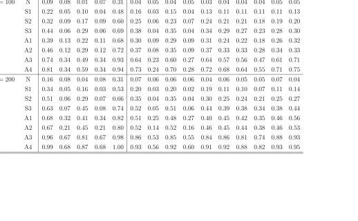
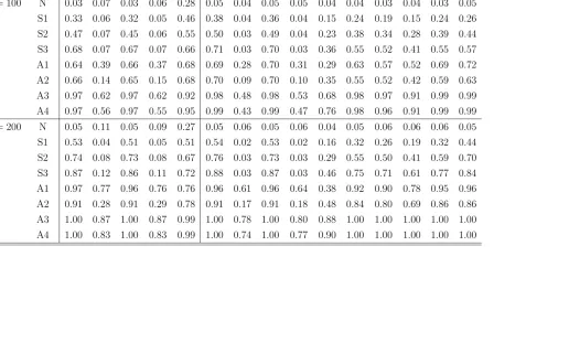
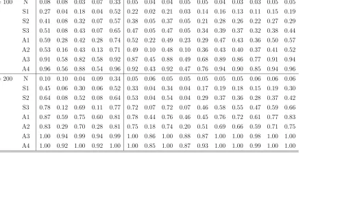
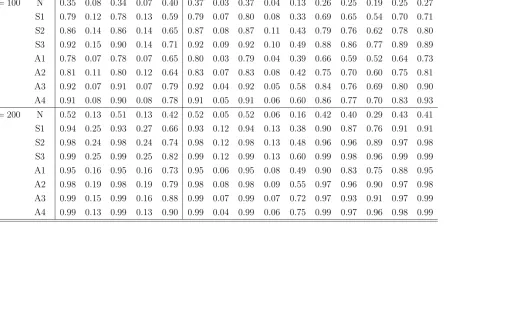
The Monte Carlo rejection frequencies of normality tests at the 5% significance level (α = 0.05) are reported in Tables 2–9. Asymptotic tests (based on J B, BN, LV,

BM, andH) rely on critical values from the relevant chi-square distribution; bootstrap tests use critical values obtained by an autoregressive sieve bootstrap procedure. The results over all design points which do not satisfy the null hypothesis are summarized graphically in the form of the box plot of the empirical rejection frequencies shown in Figure1 (bootstrap tests are indicated by the subscript B).

Inspection of the results in Tables2–4(under Gaussian innovations) and in Table5

reveals that the test based onH suffers from severe level distortion across all four data-generating mechanisms when asymptotic critical values are used. Among the remaining asymptotic tests, LV has an overall advantage under the null hypothesis for both of the sample sizes considered. TheBN and BM tests tend to be too liberal and, rather surprisingly, do not perform substantially better than the J B test, which relies on the assumption of i.i.d. observations. A possible explanation for the unsatisfactory level performance of the tests based on BN and BM may lie with the kernel estimators of the relevant long-run covariance matrices that are used in their construction. Inference procedures based on such estimators are widely reported to have poor small-sample properties, and related tests are often found to exhibit substantial level distortions in a variety of settings (see, e.g., den Haan and Levin (1997), M¨uller (2014)). As expected perhaps, bootstrap tests are generally more successful than asymptotic tests at controlling the discrepancy between the exact and nominal probabilities of Type I error. The empirical rejection frequencies of bootstrap tests are insignificantly different from the nominal 0.05 value in the vast majority of cases.

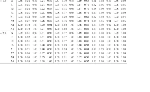
The results in Tables 2–4 (under non-Gaussian innovations) and in Tables 6–9

power-ful than theAD, CM and EP tests for some design points. The rejection frequencies of the asymptotic and bootstrapBN andBM tests have distributions which are highly positively skewed (cf. Figure1), which means that the tests are powerful only for some design points. Rather unsurprisingly, the rejection frequencies of tests improve with increasing skewness and leptokurtosis in the innovation distribution, as well as with an increasing sample size. It is worth noting that, although the asymptotic versions of some tests may appear in some cases to have similar or even higher empirical power than the corresponding bootstrap tests, such comparisons are not straightforward be-cause asymptotic tests do not generally control the probability of Type I error as well as bootstrap tests do. (The asymptotic test based on H is not included in Figure 1

because of its excessive level distortion).

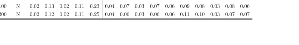
Finally, the simulation results reveal that deviations from the linearity assump-tions which underline the autoregressive sieve bootstrap procedure do not have an adverse effect on the properties of bootstrap tests. Such tests generally work well even for data that are generated by processes which are not representable as in (12) or (13). As can be seen in Table5, in the case of artificial time series from M4, the marginal dis-tribution of which is Gaussian, most bootstrap tests have rejection frequencies that do not differ substantially from the nominal level (theAD andCM tests have a tendency to over-reject). Similarly, as can be seen in Tables6–9, the bootstrap versions of tests other thanBN and BM have high rejection frequencies for data with a non-Gaussian marginal distribution generated according to the non-linear models M5–M8.

5

Summary

References

Andrews, D. W. K. (1991). Heteroskedasticity and autocorrelation consistent covariance matrix estimation. Econometrica 59, 817–858.

Andˇel, J. and P. Ranocha (2005). Stationary distribution of absolute autoregression.

Kybernetika 41, 735–742.

Babu, G. J. and C. R. Rao (2004). Goodness-of-fit tests when parameters are estimated.

Sankhy¯a 66, 63–74.

Bai, J. and S. Ng (2005). Tests for skewness, kurtosis, and normality for time series data. Journal of Business and Economic Statistics 23, 49–60.

Baringhaus, L., R. Danschke, and N. Henze (1989). Recent and classical tests for normality - a comparative study. Communications in Statistics – Simulation and Computation 18, 363–379.

Baringhaus, L. and N. Henze (1988). A consistent test for multivariate normality based on the empirical characteristic function. Metrika 35, 339–348.

Berg, A., E. Paparoditis, and D. N. Politis (2010). A bootstrap test for time series linearity. Journal of Statistical Planning and Inference 140, 3841–3857.

Bickel, P. J. and P. B¨uhlmann (1997). Closure of linear processes.Journal of Theoretical Probability 10, 445–479.

Bontemps, C. and N. Meddahi (2005). Testing normality: a GMM approach. Journal of Econometrics 124, 149–186.

Bowman, K. O. and L. R. Shenton (1975). Omnibus test contours for departures from normality based on √b1 and b2. Biometrika 62, 243–250.

Brockwell, P. J. and R. A. Davis (1991). Time Series: Theory and Methods. New York: 2nd Edition, Springer.

B¨uhlmann, P. (1997). Sieve bootstrap for time series. Bernoulli 3, 123–148.

Choi, E. and P. Hall (2000). Bootstrap confidence regions constructed from autoregres-sions of arbitrary order. Journal of the Royal Statstical Society, Ser. B 62, 461–477.

Cotter, J. (2007). Varying the VaR for unconditional and conditional environments.

Journal of International Money and Finance 26, 1338–1354.

den Haan, W. J. and A. Levin (1997). A practitioner’s guide to robust covariance matrix estimation. In G. S. Maddala and C. R. Rao (Eds.), Handbook of Statistics: Robust Inference, Volume 15, pp. 299–342. Amsterdam: North-Holland.

Durbin, J. (1973). Weak convergence of the sample distribution function when param-eters are estimated. Annals of Statistics 1, 279–290.

Epps, T. W. and L. B. Pulley (1983). A test for normality based on the empirical characteristic function. Biometrika 70, 723–726.

Hall, P. (1986). On the number of bootstrap simulations required to construct a confi-dence interval. Annals of Statistics 14, 1453–1462.

Hinich, M. J. (1982). Testing for Gaussianity and linearity of a stationary time series.

Journal of Time Series Analysis 3, 169–176.

Jarque, C. M. and A. K. Bera (1987). A test for normality of observations and regression residuals. International Statistical Review 55, 163–172.

Jim´enez-Gamero, M. D., J. Mu˜noz Garc´ıa, and R. Pino-Mej´ıas (2003). Bootstrap-ping parameter estimated degenerate U and V statistics. Statistics and Probability Letters 61, 61–70.

J¨ockel, K.-H. (1986). Finite-sample properties and asymptotic efficiency of Monte Carlo tests. Annals of Statistics 14, 336–347.

Kilian, L. and U. Demiroglu (2000). Residual-based tests for normality in autoregres-sions: asymptotic theory and simulation evidence. Journal of Business and Economic Statistics 18, 40–50.

Kojadinovic, I. and J. Yan (2012). Goodness-of-fit testing based on a weighted boot-strap: a fast large-sample alternative to the parametric bootstrap. Canadian Journal of Statistics 40, 480–500.

Kreiss, J.-P. (1992). Bootstrap procedures for AR(∞) processes. In K.-H. J¨ockel, G. Rothe, and W. Sendler (Eds.), Bootstrapping and Related Techniques, pp. 107– 113. Heidelberg: Springer-Verlag.

Kreiss, J.-P., E. Paparoditis, and D. N. Politis (2011). On the range of validity of the autoregressive sieve bootstrap. Annals of Statistics 39, 2103–2130.

Lee, S. and A. Karagrigoriou (2001). An asymptotically optimal selection of the order of a linear process. Sankhy¯a, Ser. A 63, 93–106.

Lehmann, E. L. and J. P. Romano (2005). Testing Statistical Hypotheses. New York: 3rd Edition, Springer.

Leslie, J. R., M. A. Stephens, and S. Fotopoulos (1986). Asymptotic distribution of the Shapiro–Wilk W for testing for normality. Annals of Statistics 14, 1497–1506.

Leucht, A. (2012). DegenerateU- andV-statistics under weak dependence: asymptotic theory and bootstrap consistency. Bernoulli 18, 552–585.

Leucht, A. and M. H. Neumann (2009). Consistency of general bootstrap methods for degenerate U-type and V-type statistics. Journal of Multivariate Analysis 100, 1622–1633.

Lobato, I. N. and C. Velasco (2004). A simple test of normality for time series. Econo-metric Theory 20, 671–689.

Moulines, E. and K. Choukri (1996). Time-domain procedures for testing that a station-ary time-series is Gaussian. IEEE Transactions on Signal Processing 44, 2010–2025.

M¨uller, U. K. (2014). HAC corrections for strongly autocorrelated time series. Journal of Business and Economic Statistics 32, 311–322.

Nusrat, J. and J. L. Harvill (2008). Bispectral-based goodness-of-fit tests of Gaussianity and linearity of stationary time series. Communications in Statistics – Theory and Methods 37, 3216–3227.

Paparoditis, E. (1996). Bootstrapping autoregressive and moving average parameter estimates of infinite order vector autoregressive processes. Journal of Multivariate Analysis 57, 277–296.

Paparoditis, E. and B. Streitberg (1992). Order identification statistics in stationary autoregressive moving-average models: vector autocorrelations and the bootstrap.

Journal of Time Series Analysis 13, 415–434.

Paulsen, J. and D. Tjøstheim (1985). On the estimation of residual variance and order in autoregressive time series. Journal of the Royal Statistical Society, Ser. B 47, 216–228.

Poskitt, D. S. (2007). Autoregressive approximation in nonstandard situations: the fractionally integrated and non-invertible cases. Annals of the Institute of Statistical Mathematics 59, 697–725.

Poskitt, D. S. (2008). Properties of the sieve bootstrap for fractionally integrated and non-invertible processes. Journal of Time Series Analysis 29, 224–250.

Pourahmadi, M. (2001). Foundations of Time Series Analysis and Prediction Theory. New York: Wiley.

Psaradakis, Z. (2016). Using the bootstrap to test for symmetry under unknown de-pendence. Journal of Business and Economic Statistics 34, 406–415.

Psaradakis, Z. and M. V´avra (2017). A distance test of normality for a wide class of stationary processes. Econometrics and Statistics 2, 50–60.

Ramberg, J. S. and B. W. Schmeiser (1974). An approximate method for generating asymmetric random variables. Communications of the ACM 17, 78–82.

Rom˜ao, X., R. Delgado, and A. Costa (2010). An empirical power comparison of univariate goodness-of-fit tests for normality. Journal of Statistical Computation and Simulation 80, 545–591.

Royston, P. (1992). Approximating the Shapiro–WilkW-test for non-normality. Statis-tics and Computing 2, 117–119.

Shibata, R. (1980). Asymptotically efficient selection of the order of the model for estimating parameters of a linear process. Annals of Statistics 8, 147–164.

Stein, C. (1972). A bound for the error in the normal approximation to the distribution of a sum of dependent random variables. InProceedings of the Sixth Berkeley Sympo-sium on Mathematical Statistics and Probability, Volume 2: Probability Theory, pp. 583–602. Berkeley: University of California Press.

Stephens, M. A. (1976). Asymptotic results for goodness-of-fit statistics with unknown parameters. Annals of Statistics 4, 357–369.

Stute, W., W. Gonz´ales Manteiga, and M. Presedo Quindimil (1993). Bootstrap based goodness-of-fit-tests. Metrika 40, 243–256.

Thode, H. C. (2002). Testing for Normality. New York: Marcel Dekker.

Tjøstheim, D. and J. Paulsen (1983). Bias of some commonly-used time series estimates.

Biometrika 70, 389–399; Corrigendum (1984), 71, 656.

Tong, H. (1990). Non-linear Time Series: A Dynamical System Approach. Oxford: Oxford University Press.

Yap, B. W. and C. H. Sim (2011). Comparisons of various types of normality tests.

Table 1: Innovation Distributions

λ1 λ2 λ3 λ4 skewness kurtosis

N – – – – 0.0 3.0

S1 0.000000 -1.000000 -0.080000 -0.080000 0.0 6.0

S2 0.000000 -0.397912 -0.160000 -0.160000 0.0 11.6

S3 0.000000 -1.000000 -0.240000 -0.240000 0.0 126.0

A1 0.000000 -1.000000 -0.007500 -0.030000 1.5 7.5

A2 0.000000 -1.000000 -0.100900 -0.180200 2.0 21.1

A3 0.000000 -1.000000 -0.001000 -0.130000 3.2 23.8

A4 0.000000 -1.000000 -0.000100 -0.170000 3.8 40.7

Figure 1: Empirical Rejection Frequencies of Normality Tests: Power

Table 2: Empirical Rejection Frequencies of Normality Tests Under M1

Asymptotic Tests Bootstrap Tests

sample distr. J B BN LV BM H J B BN LV BM H AD CM KS EP SW

n= 100 N 0.09 0.08 0.01 0.07 0.31 0.04 0.05 0.04 0.05 0.03 0.04 0.04 0.04 0.05 0.05

S1 0.22 0.05 0.10 0.04 0.48 0.16 0.03 0.15 0.04 0.13 0.11 0.11 0.11 0.11 0.13

S2 0.32 0.09 0.17 0.09 0.60 0.25 0.06 0.23 0.07 0.24 0.21 0.21 0.18 0.19 0.20

S3 0.44 0.06 0.29 0.06 0.69 0.38 0.04 0.35 0.04 0.34 0.29 0.27 0.23 0.28 0.30

A1 0.39 0.13 0.22 0.11 0.68 0.30 0.09 0.29 0.09 0.31 0.24 0.22 0.18 0.26 0.32

A2 0.46 0.12 0.29 0.12 0.72 0.37 0.08 0.35 0.09 0.37 0.33 0.33 0.28 0.34 0.33

A3 0.74 0.34 0.49 0.34 0.93 0.64 0.23 0.60 0.27 0.64 0.57 0.56 0.47 0.61 0.71

A4 0.81 0.34 0.59 0.34 0.94 0.73 0.24 0.70 0.28 0.72 0.68 0.64 0.55 0.71 0.75

n= 200 N 0.16 0.08 0.04 0.08 0.31 0.07 0.06 0.06 0.06 0.04 0.06 0.05 0.05 0.07 0.04

S1 0.34 0.05 0.16 0.03 0.53 0.20 0.03 0.20 0.02 0.19 0.11 0.10 0.07 0.11 0.14

S2 0.51 0.06 0.29 0.07 0.66 0.35 0.04 0.35 0.04 0.30 0.25 0.24 0.21 0.25 0.27

S3 0.63 0.07 0.45 0.08 0.74 0.52 0.05 0.51 0.06 0.44 0.39 0.38 0.34 0.38 0.44

A1 0.68 0.32 0.41 0.34 0.82 0.51 0.25 0.48 0.27 0.40 0.45 0.42 0.35 0.46 0.56

A2 0.67 0.21 0.45 0.21 0.80 0.52 0.14 0.52 0.16 0.46 0.45 0.44 0.38 0.46 0.53

A3 0.96 0.67 0.81 0.67 0.98 0.86 0.53 0.85 0.55 0.84 0.86 0.81 0.74 0.88 0.93

A4 0.99 0.68 0.87 0.68 1.00 0.93 0.56 0.92 0.60 0.91 0.92 0.88 0.82 0.93 0.95

Table 3: Empirical Rejection Frequencies of Normality Tests Under M2

Asymptotic Tests Bootstrap Tests

sample distr. J B BN LV BM H J B BN LV BM H AD CM KS EP SW

n= 100 N 0.03 0.07 0.03 0.06 0.28 0.05 0.04 0.05 0.05 0.04 0.04 0.03 0.04 0.03 0.05

S1 0.33 0.06 0.32 0.05 0.46 0.38 0.04 0.36 0.04 0.15 0.24 0.19 0.15 0.24 0.26

S2 0.47 0.07 0.45 0.06 0.55 0.50 0.03 0.49 0.04 0.23 0.38 0.34 0.28 0.39 0.44

S3 0.68 0.07 0.67 0.07 0.66 0.71 0.03 0.70 0.03 0.36 0.55 0.52 0.41 0.55 0.57

A1 0.64 0.39 0.66 0.37 0.68 0.69 0.28 0.70 0.31 0.29 0.63 0.57 0.52 0.69 0.72

A2 0.66 0.14 0.65 0.15 0.68 0.70 0.09 0.70 0.10 0.35 0.55 0.52 0.42 0.59 0.63

A3 0.97 0.62 0.97 0.62 0.92 0.98 0.48 0.98 0.53 0.68 0.98 0.97 0.91 0.99 0.99

A4 0.97 0.56 0.97 0.55 0.95 0.99 0.43 0.99 0.47 0.76 0.98 0.96 0.91 0.99 0.99

n= 200 N 0.05 0.11 0.05 0.09 0.27 0.05 0.06 0.05 0.06 0.04 0.05 0.06 0.06 0.06 0.05

S1 0.53 0.04 0.51 0.05 0.51 0.54 0.02 0.53 0.02 0.16 0.32 0.26 0.19 0.32 0.44

S2 0.74 0.08 0.73 0.08 0.67 0.76 0.03 0.73 0.03 0.29 0.55 0.50 0.41 0.59 0.70

S3 0.87 0.12 0.86 0.11 0.72 0.88 0.03 0.87 0.03 0.46 0.75 0.71 0.61 0.77 0.84

A1 0.97 0.77 0.96 0.76 0.76 0.96 0.61 0.96 0.64 0.38 0.92 0.90 0.78 0.95 0.96

A2 0.91 0.28 0.91 0.29 0.78 0.91 0.17 0.91 0.18 0.48 0.84 0.80 0.69 0.86 0.86

A3 1.00 0.87 1.00 0.87 0.99 1.00 0.78 1.00 0.80 0.88 1.00 1.00 1.00 1.00 1.00

A4 1.00 0.83 1.00 0.83 0.99 1.00 0.74 1.00 0.77 0.90 1.00 1.00 1.00 1.00 1.00

Table 4: Empirical Rejection Frequencies of Normality Tests Under M3

Asymptotic Tests Bootstrap Tests

sample distr. J B BN LV BM H J B BN LV BM H AD CM KS EP SW

n= 100 N 0.08 0.08 0.03 0.07 0.33 0.05 0.04 0.04 0.05 0.05 0.04 0.03 0.03 0.05 0.05

S1 0.27 0.04 0.18 0.04 0.52 0.22 0.02 0.21 0.03 0.14 0.16 0.13 0.11 0.15 0.19

S2 0.41 0.08 0.32 0.07 0.57 0.38 0.05 0.37 0.05 0.21 0.28 0.26 0.22 0.27 0.29

S3 0.51 0.08 0.43 0.07 0.65 0.47 0.05 0.47 0.05 0.34 0.39 0.37 0.32 0.38 0.44

A1 0.59 0.28 0.42 0.28 0.74 0.52 0.22 0.49 0.23 0.29 0.47 0.43 0.36 0.50 0.57

A2 0.53 0.16 0.43 0.13 0.71 0.49 0.10 0.48 0.10 0.36 0.43 0.40 0.37 0.41 0.52

A3 0.91 0.58 0.82 0.58 0.92 0.87 0.45 0.88 0.49 0.68 0.89 0.86 0.77 0.91 0.94

A4 0.96 0.56 0.88 0.54 0.96 0.92 0.43 0.92 0.47 0.76 0.94 0.90 0.85 0.94 0.96

n= 200 N 0.10 0.10 0.04 0.09 0.34 0.05 0.06 0.05 0.05 0.05 0.05 0.05 0.06 0.06 0.06

S1 0.45 0.06 0.30 0.06 0.52 0.33 0.04 0.34 0.04 0.17 0.19 0.18 0.15 0.19 0.30

S2 0.64 0.08 0.52 0.08 0.64 0.53 0.04 0.54 0.04 0.29 0.37 0.36 0.28 0.37 0.42

S3 0.78 0.12 0.69 0.11 0.77 0.72 0.07 0.72 0.07 0.46 0.58 0.55 0.47 0.59 0.66

A1 0.87 0.59 0.75 0.60 0.81 0.78 0.44 0.76 0.46 0.45 0.76 0.72 0.61 0.77 0.83

A2 0.83 0.29 0.70 0.28 0.81 0.75 0.18 0.74 0.20 0.51 0.69 0.66 0.59 0.71 0.75

A3 1.00 0.94 0.99 0.94 0.99 1.00 0.86 1.00 0.88 0.87 1.00 1.00 0.98 1.00 1.00

A4 1.00 0.92 1.00 0.92 1.00 1.00 0.85 1.00 0.87 0.93 1.00 1.00 0.99 1.00 1.00

Table 5: Empirical Rejection Frequencies of Normality Tests Under M4

Asymptotic Tests Bootstrap Tests

sample distr. J B BN LV BM H J B BN LV BM H AD CM KS EP SW

n= 100 N 0.02 0.13 0.02 0.11 0.23 0.04 0.07 0.03 0.07 0.06 0.09 0.08 0.03 0.08 0.06

n= 200 N 0.02 0.12 0.02 0.11 0.25 0.04 0.06 0.03 0.06 0.06 0.11 0.10 0.03 0.07 0.07

Table 6: Empirical Rejection Frequencies of Normality Tests Under M5

Asymptotic Tests Bootstrap Tests

sample distr. J B BN LV BM H J B BN LV BM H AD CM KS EP SW

n= 100 N 0.35 0.08 0.34 0.07 0.40 0.37 0.03 0.37 0.04 0.13 0.26 0.25 0.19 0.25 0.27

S1 0.79 0.12 0.78 0.13 0.59 0.79 0.07 0.80 0.08 0.33 0.69 0.65 0.54 0.70 0.71

S2 0.86 0.14 0.86 0.14 0.65 0.87 0.08 0.87 0.11 0.43 0.79 0.76 0.62 0.78 0.80

S3 0.92 0.15 0.90 0.14 0.71 0.92 0.09 0.92 0.10 0.49 0.88 0.86 0.77 0.89 0.89

A1 0.78 0.07 0.78 0.07 0.65 0.80 0.03 0.79 0.04 0.39 0.66 0.59 0.52 0.64 0.73

A2 0.81 0.11 0.80 0.12 0.64 0.83 0.07 0.83 0.08 0.42 0.75 0.70 0.60 0.75 0.81

A3 0.92 0.07 0.91 0.07 0.79 0.92 0.04 0.92 0.05 0.58 0.84 0.76 0.69 0.80 0.90

A4 0.91 0.08 0.90 0.08 0.78 0.91 0.05 0.91 0.06 0.60 0.86 0.77 0.70 0.83 0.93

n= 200 N 0.52 0.13 0.51 0.13 0.42 0.52 0.05 0.52 0.06 0.16 0.42 0.40 0.29 0.43 0.41

S1 0.94 0.25 0.93 0.27 0.66 0.93 0.12 0.94 0.13 0.38 0.90 0.87 0.76 0.91 0.91

S2 0.98 0.24 0.98 0.24 0.74 0.98 0.12 0.98 0.13 0.48 0.96 0.96 0.89 0.97 0.98

S3 0.99 0.25 0.99 0.25 0.82 0.99 0.12 0.99 0.13 0.60 0.99 0.98 0.96 0.99 0.99

A1 0.95 0.16 0.95 0.16 0.73 0.95 0.06 0.95 0.08 0.49 0.90 0.83 0.75 0.88 0.95

A2 0.98 0.19 0.98 0.19 0.79 0.98 0.08 0.98 0.09 0.55 0.97 0.96 0.90 0.97 0.98

A3 0.99 0.15 0.99 0.16 0.88 0.99 0.07 0.99 0.07 0.72 0.97 0.93 0.91 0.97 0.99

A4 0.99 0.13 0.99 0.13 0.90 0.99 0.04 0.99 0.06 0.75 0.99 0.97 0.96 0.98 0.99

Table 7: Empirical Rejection Frequencies of Normality Tests Under M6

Asymptotic Tests Bootstrap Tests

sample distr. J B BN LV BM H J B BN LV BM H AD CM KS EP SW

n= 100 N 0.86 0.24 0.85 0.24 0.86 0.87 0.19 0.87 0.19 0.68 0.91 0.92 0.86 0.88 0.90

S1 0.95 0.25 0.95 0.24 0.88 0.95 0.16 0.95 0.17 0.71 0.97 0.96 0.93 0.96 0.95

S2 0.97 0.24 0.97 0.23 0.88 0.97 0.15 0.97 0.17 0.76 0.98 0.99 0.96 0.98 0.98

S3 0.98 0.25 0.98 0.25 0.92 0.98 0.17 0.98 0.18 0.79 0.99 0.99 0.97 0.99 0.99

A1 0.93 0.33 0.93 0.32 0.87 0.93 0.20 0.93 0.21 0.69 0.92 0.92 0.89 0.92 0.94

A2 0.95 0.27 0.95 0.26 0.89 0.95 0.16 0.95 0.18 0.73 0.96 0.95 0.91 0.97 0.95

A3 1.00 0.72 1.00 0.72 0.94 1.00 0.62 1.00 0.66 0.81 1.00 0.99 0.97 1.00 1.00

A4 1.00 0.72 1.00 0.71 0.97 1.00 0.60 1.00 0.64 0.89 1.00 1.00 0.99 1.00 1.00

n= 200 N 0.99 0.31 0.99 0.31 0.96 0.99 0.17 0.99 0.19 0.81 1.00 1.00 0.99 0.99 1.00

S1 1.00 0.32 1.00 0.31 0.95 1.00 0.17 1.00 0.18 0.87 1.00 1.00 1.00 1.00 1.00

S2 1.00 0.31 1.00 0.31 0.98 1.00 0.17 1.00 0.18 0.88 1.00 1.00 1.00 1.00 1.00

S3 1.00 0.21 1.00 0.20 0.98 1.00 0.09 1.00 0.10 0.93 1.00 1.00 1.00 1.00 1.00

A1 1.00 0.71 1.00 0.70 0.96 1.00 0.53 1.00 0.55 0.84 0.99 0.99 0.99 1.00 1.00

A2 1.00 0.38 1.00 0.37 0.98 1.00 0.22 1.00 0.25 0.89 1.00 1.00 1.00 1.00 1.00

A3 1.00 0.88 1.00 0.89 1.00 1.00 0.81 1.00 0.82 0.96 1.00 1.00 1.00 1.00 1.00

A4 1.00 0.89 1.00 0.88 1.00 1.00 0.82 1.00 0.84 0.97 1.00 1.00 1.00 1.00 1.00

Table 8: Empirical Rejection Frequencies of Normality Tests Under M7

AsymptoticTests Bootstrap Tests

sample distr. J B BN LV BM H J B BN LV BM H AD CM KS EP SW

n= 100 N 0.09 0.09 0.09 0.10 0.39 0.07 0.05 0.11 0.05 0.21 0.07 0.07 0.06 0.08 0.09

S1 0.64 0.11 0.64 0.11 0.58 0.67 0.05 0.66 0.06 0.36 0.52 0.50 0.37 0.53 0.53

S2 0.79 0.14 0.79 0.14 0.63 0.80 0.07 0.80 0.09 0.44 0.73 0.70 0.61 0.75 0.80

S3 0.92 0.17 0.91 0.16 0.71 0.92 0.09 0.92 0.11 0.56 0.90 0.88 0.81 0.90 0.89

A1 0.94 0.76 0.94 0.75 0.70 0.95 0.63 0.95 0.64 0.51 0.97 0.96 0.91 0.98 0.98

A2 0.92 0.29 0.92 0.29 0.74 0.92 0.15 0.92 0.18 0.55 0.90 0.88 0.83 0.92 0.92

A3 1.00 0.91 1.00 0.90 0.93 1.00 0.83 1.00 0.85 0.82 1.00 1.00 1.00 1.00 1.00

A4 1.00 0.92 1.00 0.90 0.95 1.00 0.84 1.00 0.86 0.86 1.00 1.00 1.00 1.00 1.00

n= 200 N 0.16 0.07 0.16 0.06 0.62 0.17 0.02 0.17 0.02 0.36 0.11 0.08 0.07 0.10 0.14

S1 0.90 0.22 0.90 0.22 0.78 0.90 0.08 0.89 0.10 0.59 0.82 0.79 0.66 0.84 0.88

S2 0.97 0.27 0.97 0.27 0.84 0.98 0.12 0.98 0.14 0.70 0.96 0.95 0.92 0.96 0.96

S3 1.00 0.28 1.00 0.27 0.93 1.00 0.11 1.00 0.13 0.76 0.99 0.99 0.98 0.99 0.99

A1 1.00 0.91 1.00 0.91 0.89 1.00 0.83 1.00 0.83 0.74 1.00 1.00 0.99 1.00 1.00

A2 1.00 0.45 1.00 0.45 0.90 0.99 0.28 0.99 0.30 0.78 0.99 0.99 0.97 1.00 1.00

A3 1.00 0.96 1.00 0.97 0.98 1.00 0.93 1.00 0.94 0.93 1.00 1.00 1.00 1.00 1.00

A4 1.00 0.96 1.00 0.96 0.99 1.00 0.93 1.00 0.93 0.95 1.00 1.00 1.00 1.00 1.00

Table 9: Empirical Rejection Frequencies of Normality Tests Under M8

Asymptotic Tests Bootstrap Tests

sample distr. J B BN LV BM H J B BN LV BM H AD CM KS EP SW

n= 100 N 0.34 0.06 0.34 0.04 0.61 0.36 0.02 0.36 0.02 0.37 0.23 0.21 0.15 0.24 0.28

S1 0.63 0.08 0.63 0.08 0.69 0.66 0.05 0.66 0.06 0.48 0.56 0.54 0.45 0.58 0.63

S2 0.75 0.11 0.75 0.11 0.75 0.77 0.08 0.76 0.08 0.53 0.72 0.69 0.58 0.73 0.76

S3 0.82 0.14 0.82 0.13 0.75 0.84 0.08 0.84 0.10 0.57 0.80 0.77 0.71 0.80 0.85

A1 0.79 0.23 0.79 0.23 0.78 0.81 0.16 0.81 0.17 0.61 0.79 0.76 0.68 0.80 0.81

A2 0.80 0.17 0.80 0.18 0.77 0.82 0.09 0.82 0.11 0.59 0.80 0.78 0.67 0.80 0.82

A3 0.98 0.45 0.98 0.44 0.89 0.97 0.36 0.97 0.36 0.75 0.99 0.99 0.97 0.99 0.98

A4 0.99 0.43 0.99 0.42 0.93 0.99 0.33 0.99 0.34 0.82 0.99 0.99 0.98 1.00 1.00

n= 200 N 0.58 0.05 0.57 0.06 0.76 0.58 0.02 0.58 0.02 0.50 0.34 0.30 0.22 0.37 0.48

S1 0.88 0.17 0.88 0.16 0.85 0.89 0.07 0.89 0.08 0.65 0.83 0.79 0.69 0.83 0.87

S2 0.96 0.22 0.96 0.22 0.87 0.96 0.09 0.96 0.10 0.70 0.95 0.93 0.88 0.95 0.95

S3 0.99 0.22 0.99 0.22 0.91 0.99 0.09 0.99 0.11 0.78 0.99 0.98 0.94 0.99 0.98

A1 0.98 0.41 0.98 0.41 0.87 0.97 0.24 0.97 0.25 0.71 0.98 0.98 0.92 0.98 0.98

A2 0.98 0.28 0.98 0.29 0.90 0.98 0.14 0.98 0.16 0.77 0.98 0.97 0.95 0.98 0.97

A3 1.00 0.58 1.00 0.56 0.98 1.00 0.43 1.00 0.45 0.91 1.00 1.00 1.00 1.00 1.00

A4 1.00 0.58 1.00 0.57 0.98 1.00 0.42 1.00 0.43 0.93 1.00 1.00 1.00 1.00 1.00