GWmodel: an R package for exploring spatial heterogeneity using geographically weighted models

Gollini, Isabella and Lu, B. and Charlton, M. and Brunsdon, C. and Harris, P.

(2015) GWmodel: an R package for exploring spatial heterogeneity using

geographically weighted models. Journal of Statistical Software 63 (17),

ISSN 1548-7660.

Downloaded from:

Usage Guidelines:

Please refer to usage guidelines at or alternatively

January 2015, Volume 63, Issue 17. http://www.jstatsoft.org/

GWmodel

: An

R

Package for Exploring Spatial

Heterogeneity Using Geographically Weighted

Models

Isabella Gollini

University of Bristol

Binbin Lu

Wuhan University

Martin Charlton

NUI Maynooth

Christopher Brunsdon

NUI Maynooth

Paul Harris

Rothamsted Research

Abstract

Spatial statistics is a growing discipline providing important analytical techniques in a wide range of disciplines in the natural and social sciences. In theRpackageGWmodel, we present techniques from a particular branch of spatial statistics, termed geographi-cally weighted (GW) models. GW models suit situations when data are not described well by some global model, but where there are spatial regions where a suitably localized calibration provides a better description. The approach uses a moving window weighting technique, where localized models are found at target locations. Outputs are mapped to provide a useful exploratory tool into the nature of the data spatial heterogeneity. Cur-rently, GWmodelincludes functions for: GW summary statistics, GW principal compo-nents analysis, GW regression, and GW discriminant analysis; some of which are provided in basic and robust forms.

Keywords: geographically weighted regression, geographically weighted principal components analysis, spatial prediction, robust,Rpackage.

1. Introduction

described well by some universal or global model, but where there are spatial regions where a suitably localized model calibration provides a better description. The approach uses a moving window weighting technique, where localized models are found at target locations. Here, for an individual model at some target location, we weight all neighboring observations according to some distance-decay kernel function and then locally apply the model to this weighted data. The size of the window over which this localized model might apply is controlled by the bandwidth. Small bandwidths lead to more rapid spatial variation in the results while large bandwidths yield results increasingly close to the universal model solution. When there exists some objective function (e.g., the model can predict), a bandwidth can be found optimally, using cross-validation and related approaches.

The GW modelling paradigm has evolved to encompass many techniques; techniques that are applicable when a certain heterogeneity or non-stationarity is suspected in the study’s spatial process. Commonly, outputs or parameters of the GW model are mapped to provide a use-ful exploratory tool, which can often precede (and direct) a more traditional or sophisticated statistical analysis. Subsequent analyses can be non-spatial or spatial, where the latter can in-corporate stationary or non-stationary decisions. Notable GW models include: GW summary statistics (Brunsdon, Fotheringham, and Charlton 2002); GW principal components analysis (GW PCA, Fotheringham, Brunsdon, and Charlton 2002; Lloyd 2010a; Harris, Brunsdon, and Charlton 2011a); GW regression (Brunsdon, Fotheringham, and Charlton 1996, 1998, 1999; Leung, Mei, and Zhang 2000; Wheeler 2007); GW generalized linear models (Fother-inghamet al.2002;Nakaya, Fotheringham, Brunsdon, and Charlton 2005); GW discriminant analysis (Brunsdon, Fotheringham, and Charlton 2007); GW variograms (Harris, Charlton, and Fotheringham 2010a); GW regression kriging hybrids (Harris and Juggins 2011) and GW visualization techniques (Dykes and Brunsdon 2007).

Many of these GW models are included in the R (R Core Team 2014) package GWmodel

that we describe in this paper. Those that are not, will be incorporated at a later date. For the GW models that are included, there is a clear emphasis on data exploration. Notably,

GWmodel provides functions to conduct: (i) a GW PCA; (ii) GW regression with a local

ridge compensation (for addressing local collinearity); (iii) mixed GW regression; (iv) het-eroskedastic GW regression; (v) a GW discriminant analysis; (vi) robust and outlier-resistant GW modelling; (vii) Monte Carlo significance tests for non-stationarity; and (viii) GW mod-elling with a wide selection of distance metric and kernel weighting options. These functions extend and enhance functions for: (a) GW summary statistics; (b) basic GW regression; and (c) GW generalized linear models – GW models that are also found in thespgwrR package (Bivand, Yu, Nakaya, and Garcia-Lopez 2013). In this respect, GWmodel provides a more extensive set of GW modelling tools, within a single coherent framework (GWmodelsimilarly extends or complements thegwrrRpackage (Wheeler 2013b) with respect to GW regression and local collinearity issues). GWmodel also provides an advanced alternative to various ex-ecutable software packages that have a focus on GW regression – such as GWR3 (Charlton, Fotheringham, and Brunsdon 2003); theArcGISGW regression tool in the Spatial Statistics Toolbox (ESRI 2013); SAMfor GW regression applications in macroecology (Rangel, Diniz-Filho, and Bini 2010); andSpaceStatfor GW regression applications in health (BioMedware 2011).

kernel weighting options. Section4describes modelling with basic and robust GW summary statistics. Section5describes modelling with basic and robust GW PCA. Section 6describes modelling with basic and robust GW regression. Section 7 describes ways to address local collinearity issues when modelling with GW regression. Section8 describes how to use GW regression as a spatial predictor. Section9relates the functions of GWmodel to those found in the spgwr, gwrr and McSpatial (McMillen 2013) R packages. Section 10 concludes this work and indicates future work.

2. Data sets

The GWmodel package comes with five example data sets, these are: (i) Georgia, (ii)

LondonHP, (iii) USelect, (iv) DubVoter, and (v) EWHP. The Georgia data consists of se-lected 1990 US census variables (with n= 159) for counties in the US state of Georgia; and is fully described in Fotheringham et al. (2002). This data has been routinely used in a GW regression context for linking educational attainment with various contextual social variables (see also Griffith 2008). The data set is also available in the GWR 3 executable software package (Charltonet al. 2003) and the spgwrRpackage.

The LondonHP data is a house price data set for London, England. This data set (with

n= 372) is sampled from a 2001 house price data set, provided by the Nationwide Building Society of the UK and is combined with various hedonic contextual variables (Fotheringham

et al. 2002). The hedonic data reflect structural characteristics of the property, property construction time, property type and local household income conditions. Studies in house price markets with respect to modelling hedonic relationships has been a common application of GW regression (e.g., Kestens, Th´eriault, and Rosiers 2006;Bitter, Mulligan, and Dall’Erba 2007;P´aez, Long, and Farber 2008).

The USelect data consists of the results of the 2004 US presidential election at the county level, together with five census variables (with n = 3111). The data is a subset of that provided in (Robinson 2013). USelect is similar to that used for the visualization of GW discriminant analysis outputs in Foley and Demsar (2013); the only difference is that we specify the categorical, election results variable with three classes (instead of two): (a) Bush winner, (b) Kerry winner and (c) Borderline (for marginal winning results).

For this article’s presentation of GW models, we use as case studies, the DubVoter and EWHP data sets. The DubVoter data (with n = 322) is the main study data set and is used throughout Sections 4 to7, where key GW models are presented. This data is composed of nine percentage variables1, measuring: (1) voter turnout in the Irish 2004 D´ail elections and (2) eight characteristics of social structure (census data); for 322 Electoral Divisions (EDs) of Greater Dublin. Kavanagh, Fotheringham, and Charlton (2006) modelled this data using GW regression; with voter turnout (GenEl2004) the dependent variable (i.e., the percentage of the population in each ED who voted in the election). The eight independent variables measure the percentage of the population in each ED, with respect to:

ˆ DiffAdd: One year migrants (i.e., moved to a different address one year ago).

ˆ LARent: Local authority renters.

1_{Observe that none of the}

ˆ SC1: Social class one (high social class).

ˆ Unempl: Unemployed.

ˆ LowEduc: Without any formal educational.

ˆ Age18_24: Age group 18–24.

ˆ Age25_44: Age group 25–44.

ˆ Age45_64: Age group 45–64.

Thus the eight independent variables reflect measures of migration, public housing, high social class, unemployment, educational attainment, and three adult age groups.

The EWHP data (with n = 519) is a house price data set for England and Wales, this time sampled from 1999, but again provided by the Nationwide Building Society and combined with various hedonic contextual variables. Here for a regression fit, the dependent variable is PurPrice (what the house sold for) and the nine independent variables are: BldIntWr, BldPostW, Bld60s, Bld70s, Bld80s, TypDetch, TypSemiD, TypFlat and FlrArea. All inde-pendent variables are indicator variables (1 or 0) except forFlrArea. Section8uses this data when demonstrating GW regression as a spatial predictor; wherePurPrice is considered as a function of FlrArea(house floor area), only.

3. Distance matrix, kernel and bandwidth

A fundamental element in GW modelling is the spatial weighting function (Fotheringham

et al. 2002) that quantifies (or sets) the spatial relationship or spatial dependency between the observed variables. HereW(ui, vi) is an×n(withnthe number of observations) diagonal matrix denoting the geographical weighting of each observation point for model calibration point i at location (ui, vi). We have a different diagonal matrix for each model calibration point. There are three key elements in building this weighting matrix: (i) the type of distance, (ii) the kernel function and (iii) its bandwidth.

3.1. Selecting the distance function

Distance can be calculated in various ways and does not have to be Euclidean. An important family of distance metrics are Minkowski distances. This family includes the usual Euclidean distance having p = 2 and the Manhattan distance when p = 1 (where p is the power of the Minkowski distance). Another useful metric is the great circle distance, which finds the shortest distance between two points taking into consideration the natural curvature of the Earth. All such metrics are possible inGWmodel.

3.2. Kernel functions and bandwidth

Global Model wij = 1

Gaussian wij = exp

−1₂dij

b 2

Exponential wij = exp

−|dij|

b

Box-car wij =

1 if|dij|< b,

0 otherwise

Bi-square wij =

(1−(dij/b)2)2 if|dij|< b,

0 otherwise

Tri-cube wij =

(1−(|dij|/b)3)3 if|dij|< b, 0 otherwise

Table 1: Six kernel functions; wij is the j-th element of the diagonal of the matrix of geo-graphical weightsW(ui, vi), and dij is the distance between observationsiandj, andbis the bandwidth.

The Gaussian and exponential kernels are continuous functions of the distance between two observation points (or an observation and calibration point). The weights will be a maximum (equal to 1) for an observation at a GW model calibration point, and will decrease according to a Gaussian or exponential curve as the distance between observation/calibration points increases.

The box-car kernel is a simple discontinuous function that excludes observations that are further than some distance b from the GW model calibration point. This is equivalent to setting their weights to zero at such distances. This kernel allows for efficient computation, since only a subset of the observation points need to be included in fitting the local model at each GW model calibration point. This can be particularly useful when handling large data sets.

The bi-square and tri-cube kernels are similarly discontinuous, giving null weights to obser-vations with a distance greater thanb. However unlike a box-car kernel, they provide weights that decrease as the distance between observation/calibration points increase, up until the distanceb. Thus these are both distance-decay weighting kernels, as are Gaussian and expo-nential kernels.

Figure 1: Plot of the six kernel functions, with the bandwidth b= 1000, and wherew is the weight, anddis the distance between two observations.

3.3. Example

output of the functiongw.dist is a matrix containing in each row the value of the diagonal of the distance matrix for each observation.

R> library("GWmodel") R> data("EWHP")

R> houses.spdf <- SpatialPointsDataFrame(ewhp[, 1:2], ewhp) R> houses.spdf[1:6, ]

Easting Northing PurPrice BldIntWr BldPostW Bld60s Bld70s Bld80s TypDetch

1 599500 142200 65000 0 0 0 0 1 0

2 575400 167200 45000 0 0 0 0 0 0

3 530300 177300 50000 1 0 0 0 0 0

4 524100 170300 105000 0 0 0 0 0 0

5 426900 514600 175000 0 0 0 0 1 1

6 508000 190400 250000 0 1 0 0 0 1

TypSemiD TypFlat FlrArea

1 1 0 78.94786

2 0 1 94.36591

3 0 0 41.33153

4 0 0 92.87983

5 0 0 200.52756

6 0 0 148.60773

R> DM <- gw.dist(dp.locat = coordinates(houses.spdf)) R> DM[1:7, 1:7]

[,1] [,2] [,3] [,4] [,5] [,6] [,7]

[1,] 0.00 34724.78 77592.848 80465.956 410454.0 103419.00 236725.0 [2,] 34724.78 0.00 46217.096 51393.579 377808.2 71281.13 202563.8 [3,] 77592.85 46217.10 0.000 9350.936 352792.9 25863.10 160741.1 [4,] 80465.96 51393.58 9350.936 0.000 357757.4 25753.06 160945.0 [5,] 410454.04 377808.17 352792.928 357757.362 0.0 334189.84 232275.4 [6,] 103419.00 71281.13 25863.101 25753.058 334189.8 0.00 135411.2 [7,] 236725.01 202563.77 160741.096 160945.022 232275.4 135411.23 0.0

4. GW summary statistics

Although fairly simple to calculate and map, GW summary statistics are considered a vital pre-cursor to an application of any subsequent GW model, such as a GW PCA (Section5) or GW regression (Sections 6 to 8). For example, GW standard deviations (or GW inter-quartile ranges) will highlight areas of high variability for a given variable, areas where a subsequent application of a GW PCA or a GW regression may warrant close scrutiny. Basic and robust GW correlations provide a preliminary assessment of relationship non-stationarity between the dependent and an independent variable of a GW regression (Section 6). GW correlations also provide an assessment of local collinearity between two independent variables of a GW regression; which could then lead to the application of a locally compensated model (Section7).

4.1. Basic GW summary statistics

For attributeszandyat any locationiwherewij accords to some kernel function of Section3, definitions for a GW mean, a GW standard deviation, a GW measure of skew and a GW Pearson’s correlation coefficient are respectively:

m(zi) =

Pn

j=1wijzj Pn

j=1wij

s(zi) = v u u t

Pn

j=1wij(zj −m(zi))2 Pn

j=1wij

b(zi) =

3

v u u t

Pn

j=1wij(zj−m(zi))3

Pn

j=1wij s(zi)3

and

ρ(zi, yi) =

c(zi, yi)

s(zi)s(yi) (1)

with the GW covariance:

c(zi, yi) = Pn

j=1wij[(zj−m(zi)) (yj−m(yi))]

Pn j=1wij

4.2. Robust GW summary statistics

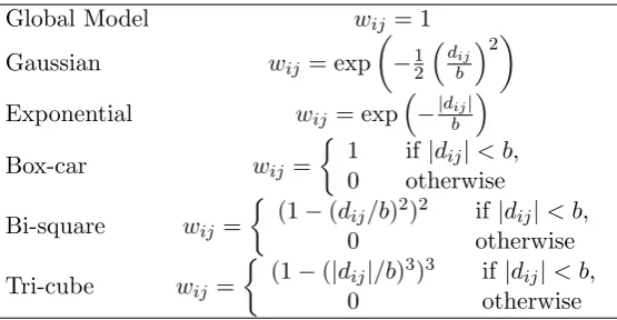
Definitions for a GW median, a GW inter-quartile range and a GW quantile imbalance, all require the calculation of GW quantiles at any locationi; the calculation of which are detailed in Brunsdonet al. (2002). Thus if we calculate GW quartiles, the GW median is the second GW quartile; and the GW inter-quartile range is the third minus the first GW quartile. The GW quantile imbalance measures the symmetry of the middle part of the local distribution and is based on the position of the GW median relative to the first and third GW quartiles. It ranges from −1 (when the median is very close to the first GW quartile) to 1 (when the median is very close to the third GW quartile), and is zero if the median bisects the first and third GW quartiles. To find a GW Spearman’s correlation coefficient, the local data for z

(a) (b)

Figure 2: (a) Basic and (b) robust GW measures of variability for GenEl2004 (turnout).

4.3. Example

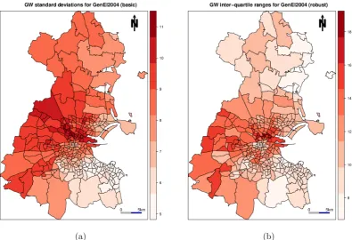
For demonstration of basic and robust GW summary statistics, we use the Dublin voter turnout data. Here we investigate the local variability in voter turnout (GenEl2004), which is the dependent variable in the regressions of Sections 6 and 7. We also investigate the local relationships between: (i) turnout and LARent and (ii) LARent and Unempl (i.e., two independent variables in the regressions of Sections6 and 7).

For any GW model calibration, it is prudent to experiment with different kernel functions. For our chosen GW summary statistics, we specify box-car and bi-square kernels; where the former relates to an un-weighted moving window, whilst the latter relates to a weighted one (from Section 3). GW models using box-car kernels are useful in that the identification of outlying relationships or structures are more likely (Lloyd and Shuttleworth 2005;Harris and Brunsdon 2010). Such calibrations more easily relate to the global model form (see Section7) and in turn, tend to provide an intuitive understanding of the degree of heterogeneity in the process. Observe that it is always possible that the spatial process is essentially homogeneous, and in such cases, the output of a GW model can confirm this.

band-(a) (b)

Figure 3: (a) Box-car and (b) bi-square specified GW correlations forGenEl2004andLARent.

width is that which provides the most accurate predictions. However, such bandwidth selec-tion funcselec-tions are not yet incorporated inGWmodel. For all other GW summary statistics, bandwidths can only be user-specified, as no objective function exists for them.

Commands to conduct our local analysis are as follows, where we use the functiongwsswith two different specifications to find our GW summary statistics. We specify box-car and bi-square kernels, each with an adaptive bandwidth ofN = 48 (approximately 15% of the data). To find robust GW summary statistics based on quantiles, thegwssfunction is specified with quantiles = TRUE(observe that we do not need to do this for our robust GW correlations).

R> data("DubVoter")

R> gw.ss.bx <- gwss(Dub.voter, vars = c("GenEl2004", "LARent", "Unempl"), + kernel = "boxcar", adaptive = TRUE, bw = 48, quantile = TRUE)

R> gw.ss.bs <- gwss(Dub.voter,vars = c("GenEl2004", "LARent", "Unempl"), + kernel = "bisquare", adaptive = TRUE, bw = 48)

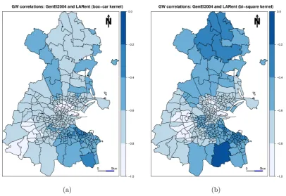
From these calibrations, we present three pairs of example visualizations: (a) basic and robust GW measures of variability forGenEl2004 (each using a box-car kernel) in Figure2; (b) box-car and bi-square specified (basic) GW correlations forGenEl2004andLARentin Figure3; and (c) basic and robust GW correlations for LARentand Unempl (each using a bi-square kernel) in Figure 4. Commands to conduct these visualizations (using palettes from RColorBrewer, Neuwirth 2011), are as follows:

R> library("RColorBrewer")

(a) (b)

Figure 4: (a) Basic and (b) robust GW correlations for LARent and Unempl.

+ offset = c(329000, 261500), scale = 4000, col = 1)

R> map.scale.1 = list("SpatialPolygonsRescale", layout.scale.bar(), + offset = c(326500, 217000), scale = 5000, col = 1,

+ fill = c("transparent", "blue"))

R> map.scale.2 = list("sp.text", c(326500, 217900), "0", cex = 0.9, col = 1) R> map.scale.3 = list("sp.text", c(331500, 217900), "5km", cex = 0.9, col = 1) R> map.layout <- list(map.na, map.scale.1, map.scale.2, map.scale.3)

R> mypalette.1 <- brewer.pal(8, "Reds") R> mypalette.2 <- brewer.pal(5, "Blues") R> mypalette.3 <- brewer.pal(6, "Greens")

R> spplot(gw.ss.bx$SDF, "GenEl2004_LSD", key.space = "right", + col.regions = mypalette.1, cuts = 7, sp.layout = map.layout, + main = "GW standard deviations for GenEl2004 (basic)")

R> spplot(gw.ss.bx$SDF, "GenEl2004_IQR", key.space = "right", + col.regions = mypalette.1, cuts = 7, sp.layout = map.layout, + main = "GW inter-quartile ranges for GenEl2004 (robust)")

R> spplot(gw.ss.bx$SDF, "Corr_GenEl2004.LARent", key.space = "right", + col.regions = mypalette.2, at = c(-1, -0.8, -0.6, -0.4, -0.2, 0), + main = "GW correlations: GenEl2004 and LARent (box-car kernel)", + sp.layout = map.layout)

+ sp.layout = map.layout)

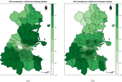
R> spplot(gw.ss.bs$SDF, "Corr_LARent.Unempl", key.space = "right", + col.regions = mypalette.3, at = c(-0.2, 0, 0.2, 0.4, 0.6, 0.8, 1), + main = "GW correlations: LARent and Unempl (basic)",

+ sp.layout = map.layout)

R> spplot(gw.ss.bs$SDF, "Spearman_rho_LARent.Unempl", key.space = "right", + col.regions = mypalette.3, at = c(-0.2, 0, 0.2, 0.4, 0.6, 0.8, 1), + main = "GW correlations: LARent and Unempl (robust)",

+ sp.layout = map.layout)

From Figure 2, we can see that turnout appears highly variable in areas of central and west Dublin. From Figure3, the relationship between turnout andLARentappears non-stationary, where this relationship is strongest in areas of central and south-west Dublin. Here turnout tends to be low while local authority renting tends to be high. From Figure4, consistently strong positive correlations betweenLARentandUnemplare found in south-west Dublin. This is precisely an area of Dublin where local collinearity in the GW regression of Section 7 is found to be strong and a cause for concern.

From these visualizations, it is clearly important to experiment with the calibration of a GW model, as subtle differences in our perception of the non-stationary effect can result by a simple altering of the specification. Experimentation with different bandwidth sizes is also important, especially in cases when an optimal bandwidth cannot be specified. Observe that all GW models are primarily viewed as exploratory spatial data analysis (ESDA) tools and as such, experimentation is a vital aspect of this.

5. GW principal components analysis

Principal components analysis (PCA) is a key method for the analysis of multivariate data (see Jolliffe 2002). A member of the unconstrained ordination family, it is commonly used to explain the covariance structure of a (high-dimensional) multivariate data set using only a few components (i.e., provide a low-dimensional alternative). The components are linear combinations of the original variables and can potentially provide a better understanding of differing sources of variation and structure in the data. These may be visualized and interpreted using associated graphics. In geographical settings, standard PCA, in which the components do not depend on location, may be replaced with a GW PCA (Fotheringhamet al.

5.1. GW PCA

More formally, for a vector of observed variablesxiat spatial locationiwith coordinates (u, v), GW PCA involves regardingxi as conditional onuandv, and making the mean vectorµand covariance matrix Σ, functions of u and v. That is, µ(u, v) and Σ(u, v) are the local mean vector and the local covariance matrix, respectively. To find the local principal components, the decomposition of the local covariance matrix provides the local eigenvalues and local eigenvectors. The product of the i-th row of the data matrix with the local eigenvectors for thei-th location provides the i-th row of local component scores. The local covariance matrix is:

Σ(u, v) =X>W(u, v)X

whereXis the data matrix (withnrows for the observations andmcolumns for the variables); and W(u, v) is a diagonal matrix of geographic weights. The local principal components at location (ui, vi) can be written as:

L(ui, vi)V(ui, vi)L(ui, vi)>= Σ(ui, vi)

whereL(ui, vi) is a matrix of local eigenvectors;V(ui, vi) is a diagonal matrix of local eigen-values; and Σ(ui, vi) is the local covariance matrix. Thus for a GW PCA with m variables, there aremcomponents,meigenvalues,msets of component scores, andmsets of component loadings at each observed location. We can also obtain eigenvalues and their associated eigen-vectors at un-observed locations, although as no data exists for these locations, we cannot obtain component scores.

5.2. Robust GW PCA

A robust GW PCA can also be specified, so as to reduce the effect of anomalous observations on its outputs. Outliers can artificially increase local variability and mask key features in local data structures. To provide a robust GW PCA, each local covariance matrix is estimated using the robust minimum covariance determinant (MCD) estimator (Rousseeuw 1985). The MCD estimator searches for a subset ofh data points that has the smallest determinant for their basic sample covariance matrix. Crucial to the robustness and efficiency of this estimator is

h, and we specify a default value of h = 0.75n, following the recommendation of Varmuza and Filzmoser(2009).

5.3. Example

For applications of PCA and GW PCA, we again use the Dublin voter turnout data, this time focussing on the eight variables: DiffAdd, LARent, SC1, Unempl, LowEduc, Age18_24, Age25_44 and Age45_64 (i.e., the independent variables of the regression fits in Sections 6 and 7). Although measured on the same scale, the variables are not of a similar magnitude. Thus, we standardize the data and specify our PCA with the covariance matrix. The same (globally) standardized data is also used in our GW PCA calibrations, which are similarly specified with (local) covariance matrices. The effect of this standardization is to make each variable have equal importance in the subsequent analysis (at least for the PCA case)2_{. The}

2

basic and robust PCA results are found using scale, princomp and covMcd functions, as follows:

R> Data.scaled <- scale(as.matrix(Dub.voter@data[, 4:11])) R> pca.basic <- princomp(Data.scaled, cor = FALSE)

R> (pca.basic$sdev^2 / sum(pca.basic$sdev^2)) * 100

Comp.1 Comp.2 Comp.3 Comp.4 Comp.5 Comp.6 Comp.7 36.084435 25.586984 11.919681 10.530373 6.890565 3.679812 3.111449

Comp.8 2.196701

R> pca.basic$loadings

Loadings:

Comp.1 Comp.2 Comp.3 Comp.4 Comp.5 Comp.6 Comp.7 Comp.8 DiffAdd 0.389 -0.444 -0.149 0.123 0.293 0.445 0.575 LARent 0.441 0.226 0.144 0.172 0.612 0.149 -0.539 0.132 SC1 -0.130 -0.576 -0.135 0.590 -0.343 -0.401 Unempl 0.361 0.462 0.189 0.197 0.670 -0.355 LowEduc 0.131 0.308 -0.362 -0.861

Age18_24 0.237 0.845 -0.359 -0.224 -0.200 Age25_44 0.436 -0.302 -0.317 -0.291 0.448 -0.177 -0.546 Age45_64 -0.493 0.118 0.179 -0.144 0.289 0.748 0.142 -0.164

R> R.COV <- covMcd(Data.scaled, cor = FALSE, alpha = 0.75)

R> pca.robust <- princomp(Data.scaled, covmat = R.COV, cor = FALSE) R> pca.robust$sdev^2 / sum(pca.robust$sdev^2)

Comp.1 Comp.2 Comp.3 Comp.4 Comp.5 0.419129445 0.326148321 0.117146840 0.055922308 0.043299600

Comp.6 Comp.7 Comp.8 0.017251964 0.014734597 0.006366926

R> pca.robust$loadings

Loadings:

Comp.1 Comp.2 Comp.3 Comp.4 Comp.5 Comp.6 Comp.7 Comp.8 DiffAdd 0.512 -0.180 0.284 -0.431 0.659

LARent -0.139 0.310 0.119 -0.932

SC1 0.559 0.591 0.121 0.368 0.284 -0.324

Unempl -0.188 -0.394 0.691 -0.201 0.442 0.307 LowEduc -0.102 -0.186 0.359 -0.895 0.149

Age18_24 -0.937 0.330

From the ‘percentage of total variance’ (PTV) results, the first three components collectively account for 73.6% and 86.2% of the variation in the data, for the basic and robust PCA, respectively. From the tables of loadings, component one would appear to represent older residents (Age45_64) in the basic PCA or represent affluent residents (SC1) in the robust PCA. Component two, appears to represent affluent residents in both the basic and robust PCA. These are whole-map statistics (Openshaw, Charlton, Wymer, and Craft 1987) and interpretations that represent a Dublin-wide average. However, it is possible that they do not represent local social structure particularly reliably. If this is the case, an application of GW PCA may be useful, which will now be demonstrated.

Kernel bandwidths for GW PCA can be found automatically using a cross-validation ap-proach, similar in nature to that used in GW regression (Section6). Details of this automated procedure are described inHarriset al.(2011a), where, a ‘leave-one-out’ cross-validation (CV) score is computed for all possible bandwidths and an optimal bandwidth relates to the small-est CV score found. With this procedure, it is currently necessary to decidea priori upon the number of components to retain (k, say), and a different optimal bandwidth results for each

k. The procedure does not yield an optimal bandwidth if all components are retained (i.e.,

m=k); in this case, the bandwidth must be user-specified. Thus for our analysis, an optimal adaptive bandwidth is found using a bi-square kernel, for both a basic and a robust GW PCA. Here,k = 3 is chosen on an a priori basis. With GWmodel, the bw.gwpca function is used in the following set of commands, where the standardized data is converted to a spatial form via theSpatialPointsDataFrame function.

R> Coords <- as.matrix(cbind(Dub.voter$X, Dub.voter$Y)) R> Data.scaled.spdf <- SpatialPointsDataFrame(Coords, + as.data.frame(Data.scaled))

R> bw.gwpca.basic <- bw.gwpca(Data.scaled.spdf, vars = colnames( + Data.scaled.spdf@data), k = 3, robust = FALSE, adaptive = TRUE) R> bw.gwpca.basic

[1] 131

R> bw.gwpca.robust <- bw.gwpca(Data.scaled.spdf, vars = colnames( + Data.scaled.spdf@data), k = 3, robust = TRUE, adaptive = TRUE) R> bw.gwpca.robust

[1] 130

Inspecting the values of bw.gwpca.basic and bw.gwpca.robust show that (very similar) optimal bandwidths ofN = 131 and N = 130 will be used to calibrate the respective basic and robust GW PCA fits. Observe that we now specify allk= 8 components, but will focus our investigations on only the first three components. This specification ensures that the variation locally accounted for by each component, is estimated correctly. The two GW PCA fits are found using thegwpcafunction as follows:

R> gwpca.basic <- gwpca(Data.scaled.spdf,

(a) (b)

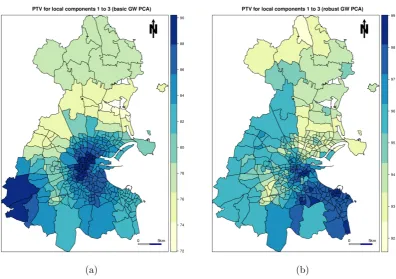
Figure 5: (a) Basic and (b) robust PTV data for the first three local components.

R> gwpca.robust <- gwpca(Data.scaled.spdf,

+ vars = colnames(Data.scaled.spdf@data), bw = bw.gwpca.robust, k = 8, + robust = TRUE, adaptive = TRUE)

The GW PCA outputs3may now be now visualized and interpreted, focusing on: (1) how data dimensionality varies spatially and (2) how the original variables influence the components. For the former, the spatial distribution of local PTV for say, the first three components can be mapped. Commands to conduct this mapping for basic and robust GW PCA outputs are as follows, where theprop.varfunction is used to find the PTV data, which is then added to the Dub.voter spatial data frame, so that it can be easily mapped using thespplot function.

R> prop.var <- function(gwpca.obj, n.components) { + return((rowSums(gwpca.obj$var[, 1:n.components]) / + rowSums(gwpca.obj$var)) * 100)

+ }

R> var.gwpca.basic <- prop.var(gwpca.basic, 3) R> var.gwpca.robust <- prop.var(gwpca.robust, 3) R> Dub.voter$var.gwpca.basic <- var.gwpca.basic R> Dub.voter$var.gwpca.robust <- var.gwpca.robust R> mypalette.4 <- brewer.pal(8, "YlGnBu")

R> spplot(Dub.voter, "var.gwpca.basic", key.space = "right", + col.regions = mypalette.4, cuts = 7, sp.layout = map.layout,

3

(a) (b)

Figure 6: (a) Basic and (b) robust GW PCA results for the winning variable on the first component. Map legends are: DiffAdd - light pink; LARent - blue; SC1 - grey; Unempl -purple; LowEduc- orange; Age18_24- green;Age25_44- brown; and Age45_64- yellow.

+ main = "PTV for local components 1 to 3 (basic GW PCA)") R> spplot(Dub.voter, "var.gwpca.robust", key.space = "right", + col.regions = mypalette.4, cuts = 7, sp.layout = map.layout, + main = "PTV for local components 1 to 3 (robust GW PCA)")

Figure 5presents the local PTV maps for the two GW PCA fits. There is clear geographical variation in the PTV data and a higher PTV is generally accounted for in the local case, than in the global case. The spatial patterns in both maps are broadly similar, with higher percentages located in the south, whilst lower percentages are located in the north. As would be expected, the robust PTV data is consistently higher than the basic PTV data. Variation in the basic PTV data is also greater than that found in the robust PTV data. Large (relative) differences between the basic and robust PTV outputs (e.g., in south-west Dublin) can be taken to indicate the existence of global or possibly, local multivariate outliers.

We can next visualize how each of the eight variables locally influence a given component, by mapping the ‘winning variable’ with the highest absolute loading. For brevity, we present such maps for the first component, only. Commands to conduct this mapping for basic and robust GW PCA outputs are as follows:

R> Dub.voter$win.item.basic <- win.item.basic R> Dub.voter$win.item.robust <- win.item.robust

R> mypalette.5 <- c("lightpink", "blue", "grey", "purple", "orange", + "green", "brown", "yellow")

R> spplot(Dub.voter, "win.item.basic", key.space = "right",

+ col.regions = mypalette.5, at = c(1, 2, 3, 4, 5, 6, 7, 8, 9),

+ main = "Winning variable: highest abs. loading on local Comp.1 (basic)", + colorkey = FALSE, sp.layout = map.layout)

R> spplot(Dub.voter, "win.item.robust", key.space = "right",

+ col.regions = mypalette.5, at = c(1, 2, 3, 4, 5, 6, 7, 8, 9),

+ main = "Winning variable: highest abs. loading on local Comp.1 (robust)", + colorkey = FALSE, sp.layout = map.layout)

Figure6presents the ‘winning variable’ maps for the two GW PCA fits, where we can observe clear geographical variation in the influence of each variable on the first component. For basic GW PCA, low educational attainment (Low_Educ) dominates in the northern and south-western EDs, whilst public housing (LARent) dominates in the EDs of central Dublin. The corresponding PCA ‘winning variable’ is Age45_64, which is clearly not dominant through-out Dublin. Variation in the results from basic GW PCA is much greater than that found with robust GW PCA (reflecting analogous results to that found with the PTV data). For robust GW PCA, Age45_64 does in fact dominate in most areas, thus reflecting a closer correspondence to the global case - but interestingly only the basic fit, and not the robust fit.

6. GW regression

6.1. Basic GW regression

The most popular GW model is GW regression (Brunsdonet al.1996,1998), where spatially-varying relationships are explored between the dependent and independent variables. Explo-ration commonly consists of mapping the resultant local regression coefficient estimates and associated (pseudo)t-values to determine evidence of non-stationarity. The basic form of the GW regression model is:

yi =βi0+

m X

k=1

βikxik+i

where yi is the dependent variable at location i; xik is the value of the kth independent variable at locationi;mis the number of independent variables;βi0 is the intercept parameter

at locationi;βik is the local regression coefficient for thekth independent variable at location

i; and i is the random error at location i.

As data are geographically weighted, nearer observations have more influence in estimating the local set of regression coefficients than observations farther away. The model measures the inherent relationships around each regression pointi, where each set of regression coefficients is estimated by a weighted least squares approach. The matrix expression for this estimation is:

ˆ

βi =

X>W(ui, vi)X −1

whereX is the matrix of the independent variables with a column of 1s for the intercept; y

is the dependent variable vector; ˆβi = (βi0, . . . , βim)> is the vector of m+ 1 local regression coefficients; and Wi is the diagonal matrix denoting the geographical weighting of each ob-served data for regression pointi at location (ui, vi). This weighting is determined by some kernel function as described in Section3.

An optimum kernel bandwidth for GW regression can be found by minimising some model fit diagnostic, such as a leave-one-out cross-validation (CV) score (Bowman 1984), which only accounts for model prediction accuracy; or the Akaike Information Criterion (AIC) (Akaike 1973), which accounts for model parsimony (i.e., a trade-off between prediction accuracy and complexity). In practice, a corrected version of the AIC is used, which unlike basic AIC is a function of sample size (Hurvich, Simonoff, and Tsai 1998). For GW regression, this entails that fits using small bandwidths receive a higher penalty (i.e., are more complex) than those using large bandwidths. Thus for a GW regression with a bandwidthb, its AICc can be found from:

AICc(b) = 2nln(ˆσ) +nln(2π) +n

n+ tr(S)

n−2−tr(S)

where n is the (local) sample size (according to b); ˆσ is the estimated standard deviation of the error term; and tr(S) denotes the trace of the hat matrix S. The hat matrix is the projection matrix from the observedy to the fitted values, ˆy.

6.2. Robust GW regression

To identify and reduce the effect of outliers in GW regression, various robust extensions have been proposed, two of which are described in Fotheringham et al. (2002). The first robust model re-fits a GW regression with a filtered data set that has been found by removing obser-vations that correspond to large externally studentized residuals of an initial GW regression fit. An externally studentized residual for each regression location iis defined as:

ri =

ei ˆ

σ−i

√

qii

whereei is the residual at location i; ˆσ−i is a leave-one-out estimate of ˆσ; and qii is the ith element of (I −S)(I −S)>. Observations are deemed outlying and filtered from the data if they have |ri| >3. The second robust model, iteratively down-weights observations that correspond to large residuals. This (non-geographical) weighting functionwr on the residual

ei is typically taken as:

wr(ei) =

  

 

1, if|ei| ≤2ˆσ

1−(|ei| −2)2 2

, if 2ˆσ <|ei|<3ˆσ

0 otherwise

Observe that both approaches have an element of subjectivity, where the filtered data ap-proach depends on the chosen residual cut-off (in this case, 3) and the iterative (automatic) approach depends on the chosen down-weighting function, with its associated cut-offs.

6.3. Example

the electorate who turned out on voting night to cast their vote in the 2004 General Election in Ireland. The dependent variable is GenEl2004 and the eight independent variables are DiffAdd,LARent,SC1,Unempl,LowEduc,Age18_24,Age25_44andAge45_64.

A global correlation analysis suggests that voter turnout is negatively associated with the independent variables, except for social class (SC1) and older adults (Age45_64). Public renters (LARent) and unemployed (Unempl) have the highest correlations (both negative), in this respect. The GW correlation analysis from Section 4 indicates that some of these relationships are non-stationary. The global regression fit to this data yields an R-squared value of 0.63 and details of this fit can be summarized as follows:

R> lm.global <- lm(GenEl2004 ~ DiffAdd + LARent + SC1 + Unempl + LowEduc + + Age18_24 + Age25_44 + Age45_64, data = Dub.voter)

R> summary(lm.global)

Coefficients:

Estimate Std. Error t value Pr(>|t|) (Intercept) 77.70467 3.93928 19.726 < 2e-16 *** DiffAdd -0.08583 0.08594 -0.999 0.3187 LARent -0.09402 0.01765 -5.326 1.92e-07 *** SC1 0.08637 0.07085 1.219 0.2238 Unempl -0.72162 0.09387 -7.687 1.96e-13 *** LowEduc -0.13073 0.43022 -0.304 0.7614 Age18_24 -0.13992 0.05480 -2.554 0.0111 * Age25_44 -0.35365 0.07450 -4.747 3.15e-06 *** Age45_64 -0.09202 0.09023 -1.020 0.3086

Next, we conduct a model specification exercise in order to help find an independent variable subset for our basic GW regression. As an aide to this task, a pseudo stepwise procedure is used that proceeds in a forward direction. The procedure can be described in the following four steps, where the results are visualized using associated plots of each model’s AICcvalues:

1. Start by calibrating all possible bivariate GW regressions by sequentially regressing a single independent variable against the dependent variable;

2. Find the best performing model which produces the minimum AICc, and permanently include the corresponding independent variable in subsequent models;

3. Sequentially introduce a variable from the remaining group of independent variables to construct new models with the permanently included independent variables, and determine the next permanently included variable from the best fitting model that has the minimum AICc;

4. Repeat step 3 until all independent variables are permanently included in the model.

Journal of Statistical Software 21

View of GWR model selection with different variables

1 2 3 ● 4 ● 5 6 7 8 ● 9 ● 10 11 12 13 14 15 ● 16 17 ● 18 19 20 21 ● 22 ● 23 24 25 26 ● 27 28 ● 29 30 ● 31 ● 32 33 ● 34 ● ₃₅

● ● 36

● ● GenEl2004 DiffAdd LARent SC1 Unempl LowEduc Age18_24 Age25_44 Age45_64 1 2 3 ● 4 ● 5 6 7 8 ● 9 ● 10 11 12 13 14 15 ● 16 17 ● 18 19 20 21 ● 22 ● 23 24 25 26 ● 27 28 ● 29 30 ● 31 ● 32 33 ● 34 ● ₃₅

● ● 36

● ● GenEl2004 DiffAdd LARent SC1 Unempl LowEduc Age18_24 Age25_44 Age45_64

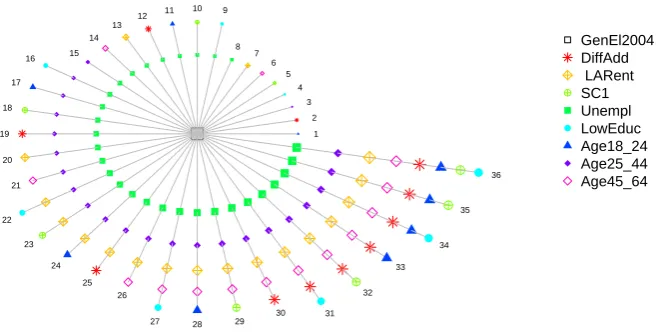
Figure 7: Model view of the stepwise specification procedure.

each GW regression fit. Alternatively, a more refined model specification exercise enables the re-calculation of an optimal bandwidth for each GW regression fit. As a demonstration, a rudimentary specification is conducted, by running the following sequence of commands. Ob-serve that a bi-square kernel is specified with a user-specified adaptive bandwidth ofN = 80.

R> DeVar <- "GenEl2004"

R> InDeVars <- c("DiffAdd"," LARent", "SC1", "Unempl", "LowEduc", + "Age18_24", "Age25_44", "Age45_64")

R> model.sel <- model.selection.gwr(DeVar, InDeVars, data = Dub.voter, + kernel = "bisquare", adaptive = TRUE, bw = 80)

R> sorted.models <- model.sort.gwr(model.sel, numVars = length(InDeVars), + ruler.vector = model.sel[[2]][,2])

R> model.list <- sorted.models[[1]]

R> model.view.gwr(DeVar, InDeVars, model.list = model.list)

R> plot(sorted.models[[2]][,2], col = "black", pch = 20, lty = 5, + main = "Alternative view of GWR model selection procedure", + ylab = "AICc", xlab = "Model number", type = "b")

Figure7presents a circle view of the 36 GW regressions (numbered 1 to 36) that result from this stepwise procedure. Here the dependent variable is located in the centre of the chart and the independent variables are represented as nodes differentiated by shapes and colors. The first independent variable that is permanently included is Unempl, the second is Age25_44, and the last isLowEduc. Figure 8 displays the corresponding AICc values from the same fits of Figure 7. The two graphs work together, explaining model performance when more and more variables are introduced. Clearly, AICc values continue to fall until all independent variables are included. Results suggest that continuing with all eight independent variables is worthwhile (at least for our user-specified bandwidth).

● ●

● ●

● ●

● ●

● ●

●

● ●

●

● ●

● ●

●

● ●

●

● ●

●

● ●

● ●

● ●

● ●

● ●

●

0 5 10 15 20 25 30 35

1800

1900

2000

2100

Alternative view of GWR model selection procedure

Model number

AICc

Figure 8: AICc values for the same 36 GW regressions of Figure7.

bandwidth to parametrize the same GW regression with the functiongwr.basic. The optimal bandwidth is found at N = 109. Commands for these operations are as follows, where the print function provides a useful report of the global and GW regression fits, with summaries of their regression coefficients, diagnostic information and F-test results (followingLeung et al.

2000). The report is designed to match the output of the GW regression v3.0 executable softwareCharltonet al. (2003).

R> bw.gwr.1 <- bw.gwr(GenEl2004 ~ DiffAdd + LARent + SC1 + Unempl + + LowEduc + Age18_24 + Age25_44 + Age45_64, data = Dub.voter, + approach = "AICc", kernel = "bisquare", adaptive = TRUE) R> bw.gwr.1

[1] 109

R> gwr.res <- gwr.basic(GenEl2004 ~ DiffAdd + LARent + SC1 + Unempl + + LowEduc + Age18_24 + Age25_44 + Age45_64, data = Dub.voter,

+ bw = bw.gwr.1, kernel = "bisquare", adaptive = TRUE, F123.test = TRUE) R> print(gwr.res)

(a) (b)

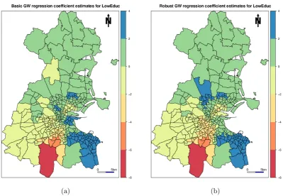
Figure 9: (a) Basic and (b) robust GW regression coefficient estimates forLowEduc.

variation, ranging from −7.67 to 3.41. Its global regression coefficient estimate is −0.13. Commands for a robust GW regression fit (the second, iterative approach) of the same model, using the same bandwidth, are also given. Here a slightly different set of coefficient estimates forLowEducresult (Figure9b), to that found with the basic fit. Evidence for relationship non-stationarity is now slightly weaker, as the robustly estimated coefficients range from−7.74 to 2.57, but the broad spatial pattern in these estimates remain largely the same.

R> names(gwr.res$SDF)

R> mypalette.6 <- brewer.pal(6, "Spectral")

R> spplot(gwr.res$SDF, "LowEduc", key.space = "right",

+ col.regions = mypalette.6, at = c(-8, -6, -4, -2, 0, 2, 4), + main = "Basic GW regression coefficient estimates for LowEduc", + sp.layout = map.layout)

R> rgwr.res <- gwr.robust(GenEl2004 ~ DiffAdd + LARent + SC1 + Unempl + + LowEduc + Age18_24 + Age25_44 + Age45_64, data = Dub.voter,

+ bw = bw.gwr.1, kernel = "bisquare", adaptive = TRUE, F123.test = TRUE) R> print(rgwr.res)

R> spplot(rgwr.res$SDF, "LowEduc", key.space = "right",

7. GW regression and addressing local collinearity

7.1. Introduction

A problem which has long been acknowledged in regression modelling is that of collinearity among the predictor (independent) variables. The effects of collinearity include a loss of precision and a loss of power in the coefficient estimates. Collinearity is potentially more of an issue in GW regression because: (i) its effects can be more pronounced with the smaller spatial samples used in each local estimation and (ii) if the data are spatially heterogeneous in terms of its correlation structure, some localities may exhibit collinearity while others may not. In both cases, collinearity may be a source of problems in GW regression even when no evidence is found for collinearity in the global model (Wheeler and Tiefelsdorf 2005;Wheeler 2007, 2013a). A further complication is that in the case of a predictor which has little local spatial variation, the possibility of collinearity with the intercept term is raised (Wheeler 2007, 2010, 2013a). Simulation studies have indicated that in the presence of collinearity, GW regression may find patterns in the coefficients where no patterns are actually present (Wheeler and Tiefelsdorf 2005;P´aez, Farber, and Wheeler 2011).

To this extent, diagnostics to investigate the nature of collinearity in a GW regression anal-ysis should always be conducted; this includes finding: (a) local correlations amongst pairs of predictors; (b) local variance inflation factors (VIFs) for each predictor; (c) local variance decomposition proportions (VDPs); and (d) local design (or cross-product) matrix condition numbers; all at the same spatial scale of each local regression of the GW regression model. Accordingly, the following rules of thumb can be taken to indicate likely local collinear-ity problems in the GW regression fit: (a) absolute local correlations greater than 0.8 for a given predictor variable pair; (b) VIFs greater than 10 for a given predictor; (c) VDPs greater than 0.5; and (d) condition numbers greater than 30. Such diagnostics and associated rules of thumb are directly taken from the global regression case (Belsley, Kuh, and Welsch 1980;O’Brien 2007) and have been proposed in a GW regression context through the works of Wheeler and Tiefelsdorf (2005); Wheeler (2007). All four diagnostics can be found and mapped using the functiongwr.collin.diagnoinGWmodeland a similar function exists in thegwrr Rpackage, see Section 9. Here it should be noted that local correlations and local VIFs cannot detect collinearity with the intercept;Wheeler(2010) provides a useful example of this. To this extent, the combined use of local VDPs and local condition numbers are su-perior diagnostics to local correlations and local VIFs for investigating collinearity (Wheeler 2007).

regression model (Wheeler 2007, 2009) and the GW lasso (Wheeler 2009). Both penalized GW models are biased estimators, providing no measures of coefficient uncertainty, but the GW lasso has the advantage in that it can also provide a local model selection function. In the presence of collinearity, both penalized GW models should provide more accurate local coefficient estimates, than that found with basic GW regression. Thus an investigation of relationship non-stationary should be more assured in this respect.

In this section, our aim is to present the use of local condition numbers as a diagnostic for local collinearity and also to relate this diagnostic to the ridge parameter of a GW ridge regression model. This relationship enables us to provide an alternative GW ridge regression to that demonstrated in Wheeler (2007). We call our new model, GW regression with a locally-compensated ridge term. This model differs to any existing GW ridge regression, in that: (A) it fits local ridge regressions with their own ridge parameters (i.e., the ridge parameter varies across space) and (B) it only fits such ridge regressions at locations where the local condition number is above a user-specified threshold. Thus a biased local estimation is not necessarily used everywhere; only at locations where collinearity is likely to be an issue. At all other locations, the usual un-biased estimator is used. GWmodel functions that we demonstrate arebw.gwr.lcr, to optimally estimate the bandwidth, and gwr.lcr, to fit the locally-compensated GW regression.

7.2. Ridge regression

A method to reduce the adverse effects of collinearity in the predictors of a linear model is ridge regression (Hoerl 1962; Hoerl and Kennard 1970). Other methods include principal components regression and partial least squares regression (Frank and Friedman 1993). In ridge regression the estimator is altered to include a small change to the values of the diagonal of the cross-product matrix. This is known as the ridge, indicated by λ in the following equation:

ˆ

β =

X>X+λI

−1

X>Y

The effect of the ridge is to increase the difference between the diagonal elements of the matrix and the off-diagonal elements. As the off-diagonal elements represent the co-variation in the predictors, the effect of the collinearity among the predictors in the estimation is lessened. The price of this is that ˆβ becomes biased, and the standard errors (and associated t-values) of the estimates are no longer available. Of interest is the value to be given to the ridge parameter;Lee(1987) presents an algorithm to find a value which yields the best predictions.

7.3. GW regression with local compensation

There exists a link between the definition of the condition number for the cross-product matrix (X>X) and the ridge parameter based on the observation that if the eigenvalues of

X>X are1, 2, . . . , p then the eigenvalues ofX>X+λI are1+λ, 2+λ, . . . , p+λ. The

condition numberκ of a square matrix is defined as 1/p, so the condition number for the ridge-adjusted matrix will be1+λ/p+λ. By re-arranging the terms, the ridge adjustment that will be required to yield a particular condition numberκisλ={(1−p)/(κ−1)} −p. Thus given the eigenvalues of the un-adjusted matrix, and the desired condition number, we can determine the value of the ridge which is required to yield that condition number.

local compensation of each local regression model, so that the local condition number never exceeds a specified value of κ. The condition numbers for the un-adjusted matrices may also be mapped to give an indication of where the analyst should take care in interpreting the results, or the local ridge parameters may also be mapped. For cases where collinearity is as much an issue in the global regression as in the GW regression; the local estimations will indicate precisely where the collinearity is a problem. The estimator for this locally compensated ridge (LCR) GW regression model is:

ˆ

β(ui, vi) =

X>W(ui, vi)X+λI(ui, vi) −1

X>W(ui, vi)Y

where λI(ui, vi) is the locally-compensated value of λat location (ui, vi). Observe that the same approach to estimating the bandwidth in the basic GW regression (Section 6) can be applied to the LCR GW regression model. For a cross-validation approach, the bandwidth is optimized to yield the best predictions. Collinearity tends to have a greater affect on the coefficient estimates rather than the predictions from the model, so in general, little is lost when using the locally-compensated form of the model. Details on this and an alternative locally-compensated GW regression can be found in Brunsdon, Charlton, and Harris(2012), where both models are performance tested within a simulation experiment.

7.4. Example

We examine the use of our local compensation approach with the same GW regression that is specified in Section 6, where voter turnout is a function of the eight predictor variables of the Dublin election data. For the corresponding global regression, the vif function in the

car package (Fox and Weisberg 2011) computes VIFs using the method outlined in Fox and Monette (1992). These global VIFs are given below and (noting their drawbacks given above) suggest that weak collinearity exists within this data.

R> library("car")

R> lm.global <- lm(GenEl2004 ~ DiffAdd + LARent + SC1 + Unempl + + LowEduc + Age18_24 + Age25_44 + Age45_64, data = Dub.voter) R> summary(lm.global)

R> vif(lm.global)

DiffAdd LARent SC1 Unempl LowEduc Age18_24 Age25_44 Age45_64 3.170044 2.167172 2.161348 2.804576 1.113033 1.259760 2.879022 2.434470

In addition, the PCA from Section5suggests collinearity betweenDiffAdd,LARent,Unempl, Age25_44, and Age45_64. As the first component accounts for some 36% of the variance in the data set, and of those components with eigenvalues greater than 1, the proportion of variance accounted for is 73.6%, we might consider removing variables with higher loadings. However for the purposes of illustration, we decide to keep the model as it is. Further global findings are of note, in that the correlation of turnout with Age45_64is positive, but the sign of the global regression coefficient is negative. Furthermore, only four of the global regression predictors are significant. Unexpected sign changes and relatively few significant variables are both indications of collinearity.

are scaled to have length 1; the condition number is the ratio of the largest to the smallest singular value of this matrix. The following code implements the BKW computations, where

X is the design matrix consisting of the predictor variables and a column of 1s.

R> X <- as.matrix(cbind(1, Dub.voter@data[, 4:11])) R> BKWcn <- function(X) {

+ p <- dim(X)[2]

+ Xscale <- sweep(X, 2, sqrt(colSums(X^2)), "/") + Xsvd <- svd(Xscale)$d

+ Xsvd[1] / Xsvd[p] + }

R> BKWcn(X)

[1] 41.06816

The BKW condition number is found to be 41.07 which is high, indicating that collinearity is at least, a global problem for this data. We can experiment by removing columns from the design matrix and test which variables appear to be the source of the collinearity. For example, entering:

R> BKWcn(X[, c(-2, -8)])

[1] 18.69237

allows us to examine the effects of removing both DiffAdd and Age25_44 as sources of collinearity. The reduction of the BKW condition number to 18.69 suggests that removing these two variables is a useful start. However, for demonstration purposes, we will persevere with the collinear (full specification) model, and now re-examine its GW regression fit, the one already fitted in Section 6. The main function to perform this collinearity assessment is gwr.lcr, where we aim to compare the coefficient estimates for the un-adjusted basic GW regression with those from a LCR GW regression.

In the first instance, we can use this function to find the global condition number (as that found with the global regression). This can be done simply by specifying a box-car kernel with a bandwidth equal to the sample size. This is equivalent to fittingnglobal models. Inspection of the results from the spatial data frame show that the condition numbers are all equal to 41.07, as hoped for. The same condition number is outputted by the ArcGISGeographically weighted Regression tool in the Spatial Statistics Toolbox (ESRI 2013). Commands to conduct this check on the behavior of the lcr.gwrfunction are as follows:

R> nobs <- dim(Dub.voter)[1]

R> lcrm1 <- gwr.lcr(GenEl2004 ~ DiffAdd + LARent + SC1 + Unempl + LowEduc + + Age18_24 + Age25_44 + Age45_64, data = Dub.voter, bw = nobs,

+ kernel = "boxcar", adaptive = TRUE) R> summary(lcrm1$SDF$Local_CN)

To obtain local condition numbers for a basic GW regression without a local compensation, we use thebw.gwr.lcrfunction to optimally estimate the bandwidth, and then gwr.lcrto estimate the local regression coefficients and the local condition numbers4. To match that of Section 6, we specify an adaptive bi-square kernel. Observe that the bandwidth for this model can be exactly the same as that obtained usingbw.gwr, the basic bandwidth function. With no local compensation (i.e., local ridges of zero), the cross-products matrices will be identical, but only provided the same optimization approach is specified. Here we specify a cross-validation (CV) approach, as the AICc approach is currently not an option in the bw.gwr.lcrfunction. Coincidently, for our basic GW regression of Section6, a bandwidth of

N = 109 results for both CV and AICc approaches. Commands to output the local condition numbers from our basic GW regression, and associated model comparisons are as follows:

R> lcrm2.bw <- bw.gwr.lcr(GenEl2004 ~ DiffAdd + LARent + SC1 + Unempl + + LowEduc + Age18_24 + Age25_44 + Age45_64, data = Dub.voter,

+ kernel = "bisquare", adaptive = TRUE) R> lcrm2.bw

[1] 109

R> lcrm2 <- gwr.lcr(GenEl2004 ~ DiffAdd + LARent + SC1 + Unempl + LowEduc + + Age18_24 + Age25_44 + Age45_64, data = Dub.voter, bw = lcrm2.bw,

+ kernel = "bisquare", adaptive = TRUE) R> summary(lcrm2$SDF$Local_CN)

Min. 1st Qu. Median Mean 3rd Qu. Max. 32.88 52.75 59.47 59.28 64.85 107.50

R> gwr.cv.bw <- bw.gwr(GenEl2004 ~ DiffAdd + LARent + SC1 + Unempl + + LowEduc + Age18_24 + Age25_44 + Age45_64, data = Dub.voter, + approach = "CV", kernel = "bisquare", adaptive = TRUE) R> gwr.cv.bw

[1] 109

R> mypalette.7 <- brewer.pal(8, "Reds")

R> spplot(lcrm2$SDF, "Local_CN", key.space = "right",

+ col.regions = mypalette.7, at = seq(30, 110, length = 9), + main = "Local condition numbers from basic GW regression", + sp.layout = map.layout)

Thus the local condition numbers can range from 32.88 to 107.50, all worryingly large every-where. Whilst the local estimations are potentially more susceptible to collinearity than the global model, we might consider removing some of the variables which cause problems globally. The maps will show where the problem is worst, and where action should be concentrated. The local condition numbers for this estimation are shown in Figure10a.

(a) (b)

Figure 10: Local condition numbers from: (a) basic GW regression and (b) before adjustment.

We can now calibrate a LCR GW regression, where the application of local ridge adjustment to each localX>W(ui, vi)X matrix, only occurs at locations where the local condition num-ber exceeds some user-specified threshold. At these locations, the local compensation forces the condition numbers not to exceed the same specified threshold. In this case, we follow convention and specify a threshold of 30. As a consquence, a local ridge term will be found at all locations, for this particular example. The lambda.adjust = TRUEand cn.thresh = 30arguments in thegwr.lcr function are used to invoke the local compensation process, as can be seen in following commands:

R> lcrm3.bw <- bw.gwr.lcr(GenEl2004 ~ DiffAdd + LARent + SC1 + Unempl + + LowEduc + Age18_24 + Age25_44 + Age45_64, data = Dub.voter,

+ kernel = "bisquare", adaptive = TRUE, lambda.adjust = TRUE, + cn.thresh = 30)

R> lcrm3.bw

[1] 157

R> lcrm3 <- gwr.lcr(GenEl2004 ~ DiffAdd + LARent + SC1+ Unempl + LowEduc + + Age18_24 + Age25_44 + Age45_64, data = Dub.voter, bw = lcrm3.bw, + kernel = "bisquare", adaptive = TRUE, lambda.adjust = TRUE, + cn.thresh = 30)

Min. 1st Qu. Median Mean 3rd Qu. Max. 34.34 47.08 53.84 52.81 58.66 73.72

R> summary(lcrm3$SDF$Local_Lambda)

Min. 1st Qu. Median Mean 3rd Qu. Max. 0.01108 0.03284 0.04038 0.03859 0.04506 0.05374

R> spplot(lcrm3$SDF, "Local_CN", key.space = "right",

+ col.regions = mypalette.7, at = seq(30, 110, length = 9), + main = "Local condition numbers before adjustment",

+ sp.layout = map.layout)

R> spplot(lcrm3$SDF, "Local_Lambda", key.space = "right",

+ col.regions = mypalette.7,cuts = 7, sp.layout = map.layout, + main = "Local ridge terms for LCR GW regression")

Observe that the bandwidth for the locally compensated GW regression is larger atN = 157, than for the un-adjusted (basic) GW regression (atN = 109). We could have specified the bandwidth from the un-adjusted model, but this would not provide the best fit. The larger bandwidth provides greater smoothing. Observe also that the local condition numbers (the Local_CN outputs) from this model are the local condition numbers before the adjustment (or compensation)5_{. They will tend to be smaller than those for the basic model because we}

are using a larger bandwidth. They will tend to that of the global model (i.e., 41.07).

TheLocal_Lambdaoutputs are the local ridge estimates used to adjust the local cross-products matrices. Both the local condition numbers and the local ridges can be mapped to show where the GW regression has applied different levels of adjustment in relation to the different levels of collinearity among the predictors. The local condition numbers are mapped in Figure10b, and the local ridges in Figure 11a for our LCR GW regression. The greatest adjustments were required in central Dublin, and in the north, south-west and south-east extremities of the study area.

Figure 11b plots the adjusted coefficient estimates forLARent from the locally compensated model, against those from the corresponding basic model. The general pattern would appear to be that the larger coefficients for the basic model are reduced in magnitude, and that the smaller coefficients are raised. The relationship is non-linear and a loess fit is shown in the plot. Commands for this comparison are as follows:

R> gwr.cv <- gwr.basic(GenEl2004 ~ DiffAdd + LARent + SC1 + Unempl + + LowEduc + Age18_24 + Age25_44 + Age45_64, data = Dub.voter + bw = gwr.cv.bw, kernel = "bisquare", adaptive = TRUE) R> small <- min(min(gwr.cv$SDF$LARent), min(lcrm3$SDF$LARent)) R> large <- max(max(gwr.cv$SDF$LARent), max(lcrm3$SDF$LARent)) R> plot(gwr.cv$SDF$LARent,lcrm3$SDF$LARent,

+ main = "LARent coefficients: basic vs. locally compensated", + xlab = "GW regression coefficient",

+ ylab = "LCR GW regression coefficient",

+ xlim = c(small, large), ylim = c(small, large))

(a) ●● ●● ● ● ● ● ● ● ● ● ●● ● ● ● ● ●● ● ●● ● ● ● ●●● ●●●●●● ● ● ● ● ● ●●● ● ● ● ●● ● ● ● ● ● ● ● ● ●● ● ● ● ● ● ● ● ●●● ● ● ● ● ● ●●● ● ● ● ●●●●● ●● ● ●● ● ●●● ● ● ●● ●●● ● ●● ● ● ● ● ●● ● ● ● ● ● ● ● ●● ●●● ●●● ● ● ● ● ● ● ● ● ● ● ● ● ● ● ● ●● ● ● ●● ● ● ● ● ●● ● ● ● ●● ● ● ● ● ● ● ● ● ● ● ●● ● ● ● ● ● ● ● ● ● ● ● ● ●● ● ● ● ● ● ● ● ● ● ● ● ● ● ● ● ● ● ● ● ● ● ● ● ● ● ● ● ● ● ● ● ● ● ● ● ● ● ● ● ● ● ● ● ● ● ● ● ● ● ● ● ● ● ● ● ● ●●●● ● ● ● ● ●●● ● ● ● ● ● ● ● ●● ● ● ● ● ● ● ● ● ● ● ● ● ● ● ● ● ● ● ● ● ● ● ● ● ●● ● ● ●●● ● ● ● ● ● ● ●●● ● ●● ● ● ● ● ● ● ● ● ● ● ● ● ● ● ● ● ● ● ● ● ●

−0.20 −0.15 −0.10 −0.05 0.00 0.05 0.10

−0.20 −0.15 −0.10 −0.05 0.00 0.05 0.10

LARent coefficients: Basic vs. LCR

GW regression coefficient

LCR GW regression coefficient

(b)

Figure 11: (a) Local ridge terms and (b) comparison of coefficient estimates forLARent.

R> lines(lowess(gwr.cv$SDF$LARent, lcrm3$SDF$LARent), col = "blue") R> abline(0, 1, col = "gray60")

Model building with collinear data

If we explore the local condition numbers for models with different structures, it may be possible to build GW regression models which avoid collinearity. Here, we code a function to calibrate and then estimate a basic (un-adjusted) GW regression. This function can then be used to assess various forms of the model, where the output each time is a vector of local condition numbers for the model that has been fitted. This function is presented as follows, together with an example model run.

R> test.CN <- function(model, data) {

+ lcrmx.bw <- bw.gwr.lcr(model, data = data, kernel = "bisquare", + adaptive = TRUE)

+ print(model) + print(lcrmx.bw)

+ lcrmx <- gwr.lcr(model, data = data, bw = lcrmx.bw, + kernel = "bisquare", adaptive = TRUE)

+ print(summary(lcrmx$SDF$Local_CN)) + lcrmx$SDF$Local_CN

+ }

● ● ● ● ● ● ● ● ● ● ● ● ● ● ● ● ● ● ● ● ● ● ● ● ● ● ● ● ● ● ● ● ● ● ● ● ● ● ● ● ● ● ● ● ● ● ● ● ● ● ● ● ● ● ● ● ● ● ● ● ● ● ● ● ● ● ● ● ● ● ● ● ● ● ● ● ● ● ●

ALL DA LA SC Un LE A18 A25 A45 DA+1 LA+2

20

40

60

80

100

Distribution of local condition numbers from 11 different model specs.

Figure 12: Distribution of local condition numbers from 11 different GW regression fits.

R> model <- as.formula(GenEl2004 ~ DiffAdd + LARent + SC1 + Unempl + + LowEduc + Age18_24 + Age25_44 + Age45_64)

R> AllD <- test.CN(model, data)

On using this function with eleven different GW regression models, Figure 12 shows the boxplots of the local condition numbers from GW regressions with: (i) all variables (ALL), (ii) removing each variable in turn (DiffAdd, LARent, SC1, Unempl, LowEduc, Age18_24, Age25_44, Age45_64), (iii) removing DiffAdd and Age45_64 together, and (iv) removing LARent, Age25_44 and Age45_64 together. The last grouping was suggested by the output of the global PCA from Section 5. Removing variables individually has little effect on the local condition number distributions, although removing the last two age variables induces a noticeable drop. Removing the most collinear variables produces a model where no local condition number is above 30.

Figure 13: Scatterplot matrix of local condition numbers from 11 different GW regression fits.

7.5. LCR GW regression vs. previous penalized GW regression models

short-coming of GWRR and suggested the use of local ridge terms (Wheeler 2007, p.2480), but provided no details on such a model’s implemention. Thus the advance for LCR-GWR is the actual implementation of a such a model, and in particular, the relating of the local condition number to the local ridge parameter (Section7.3).

LCR-GWR should not only be placed in context with GWRR, but also the GW lasso (GWL). Ridge regression and the lasso (Tibshirani 1996) both penalize or shrink regression coefficients, so as to reduce collinearity effects, where the lasso shrinks the least significant coefficents to zero, and in doing so, additionally (and simultaneously) provides a model selection function. Wheeler (2009) provides two versions of GWL; one that estimates a single (global) lasso parameter to control coefficient shrinkage (GWL-global), and one that estimates multiple (local) lasso parameters (GWL-local). Thus GWL-global can be viewed as an alternative to GWRR (as both are globally-focused), whilst GWL-local can be viewed as an alternative to LCR-GWR (as both are locally-focused).

A simple way to demonstrate the differences between the competing models is to run them (togther with a basic GW regression), using the same data and the same kernel weighting specification. Here the functions,gwrr.estandgwl.estfrom thegwrrRpackage are needed to fit the GWRR and GWL models, respectively. Correspondence with the author of gwrr

indicated that gwl.est only fits GWL-local models, and that an option for GWL-global is not provided. Furthermore,gwrr.est,gwl.estandgwr.est(a basic GW regression function ingwrr), only allow for fixed bandwidths with Gaussian or exponential kernel functions (see Section 9). As the bandwidth for GWL-local is optimally estimated (via cross-validation) within thegwl.est function, and cannot be user-specified, we use this particular bandwidth for all models. Thus, only GWL-local will be correctly specified with respect to its weighting function. For a data set, we choose the columbusneighborhood crime rate data available in

gwrr.

Commands to conduct this rudimentary comparison are given below, where an exponential kernel bandwidth of 1.68 is used for all models. For GWRR and LCR-GWR, only the latter provides local ridges, 16 of which are non-zero (as their corresponding local condition numbers are above 30). The only outputs that are directly comparable between all four models, are the local regression coefficients themselves. For example, if we view the coefficients forincome, 26 are zero with GWL-local, indicating that this variable is not needed in the corresponding local regressions. If we compare the income coefficients for the penalized models with those from the basic model, both GWRR and GWL-local apply some form of penalty at all locations, whereas LCR-GWR only penalizes at certain (in this case, 16) locations. Thus as would be expected, coefficients from the basic GW regression have the strongest correlation with those from the LCR-GWR model. An objective and detailed comparison of all such penalized models, using simulated data, is a subject of our current research (Brunsdonet al. 2012).

R> library("gwrr") R> data("columbus")

R> locs <- cbind(columbus$x, columbus$y)

R> columbus.spdf <- SpatialPointsDataFrame(locs, columbus)

R> gwl.comp <- gwl.est(crime ~ income + houseval, locs, columbus, "exp") R> gwl.comp$phi