Speech Enhancement using Affine Projection Algorithm
and Normalized Kernel Affine Projection Algorithm
Kavita R. Jadhav
Dept. of Electronics and Telecommunication G. H. Raisoni Institute of Engineering and Technology,
Pune, India
Mrinal R. Bachute
Dept. of Electronics and Telecommunication G. H. Raisoni Institute of Engineering and Technology,
Pune, India
R. D. Kharadkar,
Ph.D Dept. of Electronics andTelecommunication G. H. Raisoni Institute of Engineering and Technology,
Pune, India
ABSTRACT
The aim of the Speech Enhancement system is to improve the quality of noisy speech signal. This paper emphasize on enhancement of noisy speech by using Affine Projection Algorithm (APA) and Kernel Affine Projection Algorithm (KAPA). Noise is present everywhere in the environment, So Kernel adaptive filters are used to enhance noisy speech signal and shows the good improvement in increasing the Signal to Noise Ratio (SNR) and Mean square error (MSE). The computer simulations are performed using NOIZEUS speech corpus for different SNR values using Affine projection (APA), Kernel Affine projection (KAPA), Recursive least square (RLS), Kernel least mean square (KLMS) and their performance is compared.
Keywords
Speech enhancement, APA, KAPA, RKHS, MSE, SNR.
1.
INTRODUCTION
Adaptive filtering is an significant area of digital signal processing [1] Adaptive filters work on the principle of estimating a noisy signal by minimizing an objective error function, usually the mean error between the filter output signal and a desired signal. Adaptive filters are used for estimation and identification of non-stationary signals, channels and systems or in applications where a sample-by-sample adaptation of a process and/or a low processing delay is required. NLMS and RLS algorithms are widely applied adaptive algorithms for noise cancellation [2].
Kernel adaptive filters are linear adaptive filters in Reproducing kernel Hilbert spaces (RKHS). Kernel adaptive filters include kernel least mean square, kernel affine projection algorithms, kernel recursive least squares, extended kernel recursive least squares and kernel Kalman filter.
2.
SPEECH ENHANCEMENT
Speech enhancement is a challenging area of resources. Speech enhancement is used in many applications like military, speech recognition, cellular environments, telecommunication, etc. A speech enhancement reduces noise and improves speech signal quality and intelligibility. Speech enhancement is a difficult problem mainly for two reasons [1] 1. The state and characteristics of the noise signal can change not only dramatically or abruptly in time but also to find related algorithms that really works in the environmental condition.
2. For each application, performance measure can also be different. The Fig1 shows the basic idea of speech enhancement.
[image:1.595.319.544.266.381.2]Various techniques are modeled for the purpose to get better the speech signal-to noise ratio and the performances depend on superiority and precision of the processed speech signal.
Fig. 1. Basic Speech Enhancement
3.
ADAPTIVE FILTERS
Adaptive filters are required for unrevealedstable provisions or displeased specifications by time invariant filters. Adaptive filters have been effective approaches for speech enhancement for past decade. The traditional programs of controlled adaptive filters rely on error-correction for their adaptive learning ability[2]. Adaptive filter has lower processing delay[3]and fast tracking of time-varying environments. The limited computational power of linear learning machines was highlighted by Minsky and Papert [1969] in their famous work on Perceptrons.
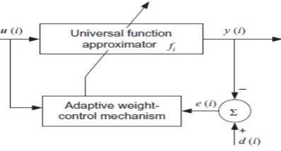
Fig. 2. Structure of nonlinear adaptive filter
An adaptive filter is defined as
yi = wiui (1) Where, i is the time index, u is the filter input, y is the filter
[image:1.595.332.531.532.639.2]The following assumptions are made:
Input signal u(i) = desired signal d(i) + interfering noise v(i)
ui = di + vi (2) The function approximator is having a Finite Impulse
Response (FIR) structure which has the impulse response is equal to the filter defined as
wi = [wi0, wi1, … . wip] (3)
The difference between the anticipated and the projected signal is the error signal
ei = di − yi (4) The function approximator will estimates the desired signal by
convolution process.
fixed- filter approximation step,
yi = wi ∗ ui(5) Function approximator updates its coefficients at every instant of time.
wi + 1 = wi + Δwi (6)
Where ∆ Wi is a correction factor for the filter coefficients
3.1
Affine Projection Algorithm (APA)
Affine Projection algorithm (APA) [5] is derived as aoverview of the NLMS algorithm. The affine projection algorithm is an adaptive filter whose persistence is to iteratively estimate the adaptive filter weights so that a function of the error signal e[n] is minimized. In APA, the projections are made in multiple dimensions and in NLMS one dimension. As increasing the projection dimension, increases the convergence rate of the tap weight vector, so that finally an increased computational complexity [5]. Let d (desired signal) be a zero-mean scalar-valued random variable[1][5] and let u (noisy) be a zero-mean L × 1 random variable with a positive-definite covariance matrix Ru = E[uuT ][1]. The cross-covariance vector of d and u is denoted by rdu = E[du]. The weight vector w that solvesMinw E |d– wTu|2 (7) is given by w0 = Ru -1 rdu [6].
Several methods that approximate ‘w’ iteratively. For example, the common gradient method
w(0) = initial guess;
wi = wi − 1 + η[rdu − Ruwi − 1] (8) Or the regularized Newton’s recursion,
w(0) = initial guess;
wi = wi − 1 + ηRu + εI − −1[rdu − Ruwi − 1]
(9) Where ɛ is a small progressive regularization factor and η is the step size. The covariance matrix and the cross-covariance vector are replaced by stochastic-gradient method. The trade-off is convergence performance, computation complexity and steady-state behavior [6].
Assuming that we have access to random variables (d and u)
The Least-mean-square (LMS)[5] algorithm simply uses the instantaneous values for approximations ˆRu = u(i)u(i)T and ˆrdu = d(i)u(i). The corresponding steepest-descent recursion (8) and Newton’s recursion (9) become
$i = wi − 1 + ηui[di − uîTwi − 1] (10) The affine projection algorithm however employs better approximations. Specifically, the approximations Ru and rdu are replaced by the instantaneous approximations from the K most recent regressors and observations. Denoting
U(i) = [u(i − K + 1), ..., u(i)] LxK and d(i) = [d(i − K + 1), . . . , d(i)]
ˆRu = (1/K)U(i)U(i)T and ˆrdu = (1/K) U(i)d(i) (11)
wi = wi − 1 + ηUi[di − UîTwi − 1] (12)
3.2
Normalized Affine Projection
Algorithm (NAPA)
The normalized affine projection algorithm becomes
wi = wi − 1 + η'Uı)TUi + εI* − 1Ui[di − UîTwi − 1] (13)
and (13), by the matrix inversion lemma, is equivalent to [6]
wi = wi − 1 + ηUi'Uı)TUi + εI* − 1[di − UîTwi − 1] (14)
It plays a very significant role in the source of kernel extensions. We call recursion (12) APA and recursion (14) normalized APA.
4.
KERNEL ADAPTIVE FILTERS
The main idea of kernel method is, the input data is transformed, to a high dimensional feature space through a reproducing kernel such that the innermost product operation can be computed efficiently in the feature space through the kernel evaluations [7]. After that an appropriate linear methods are subsequently applied on the transformed data. As long as an algorithm can be formulated, there is no call to perform computations in the high dimensional feature space. This is the main advantage Kernel Adaptive Filter [4].
4.1
Kernel Affine Projection Algorithm
(KAPA)
A kernel [4] is a symmetric, constant, positive-definite function k: U x U→R. U is the input domain, a compact subset of RL. The commonly used kernels include the Gaussian kernel (15) and the polynomial kernel (16):
ku. u, = exp −a/|u − u,|/ ̂2 (15)
ku, u, = u0Tu,+ 1̂p (16)
Algorithm Initialization: Learning step :-
For n = max(1, i − K + 1) to k do % evaluate outputs of the current network
yk, n = 1 ajk − 1kn, j
345
675
k is the kernel function (19). % Computer errors
ei, n = di − yi, n (20) % Update the min(i,K) most recent units
ani = ani − 1 + ηei, n (21) End for
if i > K then
% Keep the remaining For n = 1 to i− K do
5.
RELATED WORK
Linear Adaptive Filters: The earliest work on adaptive filters may be traced back to the late 1950s, during which time many researchers were working independently on different applications of such filters. As a result, the LMS emerged as a simple and effective algorithm for the operation of adaptive transversal filters.
Another important algorithm in adaptive filtering theory is the RLS algorithm. The original paper on the standard RLS algorithm is that of Plackett [1950], Godard first used Kalman filter theory successfully to solve adaptive filtering problems, which is known in the literature as the Godard algorithm. Then, Sayed and Kailath [1994] established an exact relationship between the RLS algorithm and Kalman filter theory, thereby laying the groundwork for how to develop the vast literature on Kalman filters for solving linear adaptive filtering problems.
The EX - RLS algorithm was first presented in Haykin et al. [1997]. It is derived as an improvement over the RLS algorithm in terms of tracking ability in non-stationary signal processing. The Kalman filter is a special case while derived from the view of adaptive signal processing. The Kalman filter is used in a wide range of engineering applications from radar to navigation, and it is an important topic in control theory and control systems engineering. A highlight application of the Kalman filter is perhaps its incorporation in the Apollo navigation computer. Two excellent textbooks for linear adaptive filtering were authored by Haykin [2002] and Sayed [2003].
Kernel Methods: The idea of using kernel functions as inner products in a feature space was introduced into machine learning by the work of Aizerman et al. [1964] on the method of potential functions. Schölkopf et al. [1998] derived the first unsupervised learning algorithm in reproducing kernel Hilbert space by introducing the kernel principal components analysis. The description of kernel Fisher discriminant analysis can be found in Mika et al. [1999]. The use of kernels for function approximation dates back to Aronszajn [1950]. Then, Wahba [1990] systematically studied reproducing kernels in approximation and regularization theory.
6.
EXPERIMENTAL RESULTS
[image:3.595.317.542.207.339.2]In this section, proposed work examines the performance of the KAPA and APA algorithms for speech enhancement at various signal-to-noise ratios of different noise conditions. The step size used for both the APA and KAPA is 0.2. There were collected the separate noise corpus from NOIZEUS [8] for proposed work and added to the clean Speech signals for the experimentation. At different noisy levels, performances of these evaluated for speech enhancement. Babble noise, Airport noise, Car noise, Restaurant noise, and Station noise at 0, 5, 10, and 15 dB SNR were experimented. For this proposed system, a total of 20 datasets were generated.
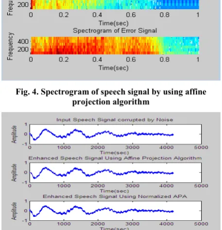
[image:3.595.315.542.375.534.2]Fig. 3. The speech signal is corrupted by noise which is enhanced by affine projection algorithm
[image:3.595.314.543.448.685.2]Fig. 4. Spectrogram of speech signal by using affine projection algorithm
Fig. 6. Spectrogram signal is enhanced by normalized affine projection algorithm
Fig. 7. Signal is enhanced by kernel affine projection algorithm
7.
PERFORMANCE ANALYSIS
The adaptive filter minimizes the error signal e(i).It is depends only on adaptive filter length, adaptive algorithm and the nature of the signal. Performance is measured on the basis of MSE and SNR
7.1
Signal to Noise Ratio (SNR)
Signal to Noise Ratio (SNR) is defined as the ratio of power between the signal and the unwanted noise. SNR is calculated using the formula
S
N =nn:;<=>?@>A;B
Speech enhancement process is to obtain high SNR ie it gives better performance.
7.2
Mean Square Error (MSE)
To quantify the difference between the values implied by an estimator and the true values of the quantity being estimated. MSE is defined as,
MSE =1n 1Yı̂ − Yî2
=
;75
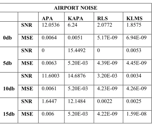
Table 1.Comparison of SNR and MSE values for APA, KAPA, RLS, KLMS algorithmsfor Airport noise at o, 5,
10, and 15 dB
AIRPORT NOISE
APA KAPA RLS KLMS
0db
SNR 12.0536 6.24 2.0772 1.8575
MSE 0.0064 0.0051 5.17E-09 6.94E-09
5db
SNR 0 15.4492 0 0.0053
MSE 0.0063 5.20E-03 4.39E-09 4.45E-09
10db
SNR 11.6003 14.6876 3.20E-03 0.0034
MSE 0.0061 5.20E-03 4.23E-09 4.26E-09
15db
SNR 1.6447 12.1484 0.0022 0.0025
[image:4.595.307.557.104.309.2]MSE 0.006 5.20E-03 4.22E-09 1.59E-08
Table 2.Comparison of SNR and MSE values for APA, KAPA, RLS, KLMS algorithms for Car noise at o, 5, 10,
and 15 dB
CAR NOISE
APA KAPA RLS KLMS
0db
SNR 2.0289 19.7016 2.1897 0.6499
MSE 0.0071 5.10E-03 5.47E-09 6.58E-09
5db
SNR 5.0251 22.9721 5.9089 6.6586
MSE 0.0062 5.20E-03 4.63E-09 4.40E-09
10db
SNR 0 18.2361 1.70E-02 0.0172
MSE 0.0063 5.20E-03 4.29E-09 4.56E-09
15db
SNR 2.5186 13.4776 2.6001 2.452
MSE 0.0059 5.20E-03 4.10E-09 4.19E-09
Table 3.Comparison of SNR and MSE values for APA, KAPA, RLS, KLMS algorithms forBabble noise at o, 5,
10, and 15 dB
BABBLE NOISE
APA KAPA RLS KLMS
0db
SNR 9.5350 19.4909 6.7305 4.8235
MSE 0.0066 5.10E-03 5.67E-09 1.24E-07
5db
SNR 0 1.58E+01 0.0027 0.0025
MSE 0.0061 5.20E-03 4.53E-09 2.71E-08
[image:4.595.53.273.247.424.2]15db
SNR 2.9918 11.5388 0.0034 3.50E-03
[image:5.595.45.547.65.771.2]MSE 0.0059 5.20E-03 4.17E-09 4.15E-09
Table 4.Comparison of SNR and MSE values for APA, KAPA, RLS, KLMS algorithms forRestaurant noise at o,
5, 10, and 15 dB
RESTAURANT NOISE
APA KAPA RLS KLMS
0db
SNR 16.1604 1.2884 0 0.0012
MSE 0.0083 5.10E-03 6.61E-09 8.01E-08
5db
SNR 14.6293 13.8087 7.2018 7.0069
MSE 0.0063 0.0052 4.48E-09 2.59E-08
10db
SNR 6.6445 12.3165 0.0019 0.0019
MSE 0.0061 0.0052 4.33E-09 4.37E-09
15db
SNR 0.5471 17.8879 0.0037 0.0037
MSE 0.006 0.0052 4.12E-09 4.12E-09
Table 5.Comparison of SNR and MSE values for APA, KAPA, RLS, KLMS algorithms forStation noise at o, 5,
10, and 15 dB
STATION NOISE
APA KAPA RLS KLMS
0db
SNR 13.1156 13.0344 1.5901 1.6264
MSE 0.0098 5.10E-03 9.19E-09 2.59E-08
5db
SNR 3.6096 30.0286 8.6215 8.0056
MSE 0.0062 1.04E-06 4.53E-09 4.93E-09
10db
SNR 7.221 13.6655 0.0107 0.0105
MSE 0.006 0.0052 4.16E-09 5.65E-09
15db
SNR 0 15.4816 0.0024 0.0025
MSE 0.006 5.20E-03 4.11E-09 4.16E-09
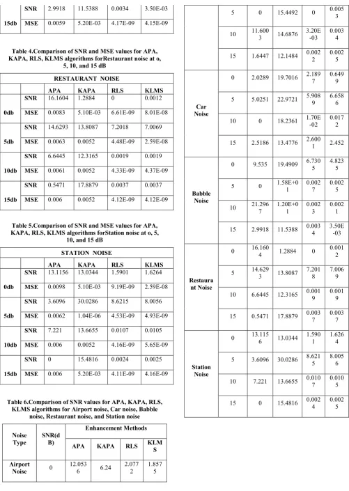
Table 6.Comparison of SNR values for APA, KAPA, RLS, KLMS algorithms for Airport noise, Car noise, Babble
noise, Restaurant noise, and Station noise
Noise Type
SNR(d B)
Enhancement Methods
APA KAPA RLS KLM S
Airport Noise 0
12.053
6 6.24
2.077 2
1.857 5
5 0 15.4492 0 0.005
3
10 11.600
3 14.6876 3.20E
-03
0.003 4
15 1.6447 12.1484 0.002 2
0.002 5
Car Noise
0 2.0289 19.7016 2.189 7
0.649 9
5 5.0251 22.9721 5.908 9
6.658 6
10 0 18.2361 1.70E -02
0.017 2
15 2.5186 13.4776 2.600
1 2.452
Babble Noise
0 9.535 19.4909 6.730 5
4.823 5
5 0 1.58E+0
1
0.002 7
0.002 5
10 21.296 7 1.20E+0 1 0.002 3 0.002 1
15 2.9918 11.5388 0.003 4
3.50E -03
Restaura nt Noise
0 16.160
4 1.2884 0
0.001 2
5 14.629
3 13.8087 7.201
8
7.006 9
10 6.6445 12.3165 0.001 9
0.001 9
15 0.5471 17.8879 0.003 7
0.003 7
Station Noise
0 13.115
6 13.0344 1.590
1
1.626 4
5 3.6096 30.0286 8.621 5
8.005 6
10 7.221 13.6655 0.010 7
0.010 5
15 0 15.4816 0.002 4
Graphical Representation
1.
Airport Noise
2.
Car Noise
3.
Babble noise
4.
Restaurant noise
5.
Station noise
This is the graphical representation of comparison of SNR values for above Airport, Babble noise, Car noise, Restaurant noise, Station noise. From graphs, proposed systemshows that KAPA gives the better result as compared with APA at different SNR value. Similarly proposed system has higher performance of SNR and lowers the MSE value for Airport, Car, Station, Babble, Restaurant noises etc.
8.
CONCLUSION
The KAPA algorithm performs much better results compared to APA, RLS, KLMS in terms of SNR and MSE values. In this paper, proposed system shows a better improvement in removal of background noise .The experimental results had shown that when compared to the other algorithms it provides better noise reduction at faster converging speed, improved speech quality and intelligibility. In future,proposed system gives high quality speech signal without any noise distortion.
9.
REFERENCES
[1] Bolimera Ravi, Lim, T.Kishore Kumar, "Speech enhancement using kernel and normalized affine projection algorithm,” Signal and image Processing, vol.4, August2013.
[4] N. Aronszajn, “Theory of reproducing kernels,” Trans. Amer. Math. Soc., vol. 68, pp. 337–404, 1950.
[5] Jose C. Principe, Weifeng Liu, and Simon Haykin "Kernel Adaptive Filtering: A Comprehensive Introduction", Wiley, March 2010.
[6] A. Sayed, Fundamentals of Adaptive Filtering. New York: Wiley, 2003
[7] W. Liu, P. Pokharel, and J. C. Principe, “The kernel least mean square algorithm,” IEEE Transactions on Signal Processing, vol. 56, 2008.