Software Assessment Parameter Optimization using
Genetic Algorithm
Neha Sharma
Technocrats Institute of Technology,
Bhopal, Madhya Pradesh, India
Amit Sinhal
Technocrats Institute of Technology,
Bhopal, Madhya Pradesh, India
Bhupendra Verma,Ph.D
Technocrats Institute of Technology (Excellence), Bhopal, Madhya Pradesh, India
ABSTRACT
Software assessment of a project is a key aspect for the prediction of the cost, duration and the expertise required for the project. An efficient optimization algorithm is urgently needed. In this paper, we analyze the genetic algorithm (GA) technique for the development of a software assessment model for the NASA software project dataset. The simulation is performed using MATLAB environment and the results are tested on the basis of measures such as MMRE, MdMRE, MMER, Prediction Accuracy (25%) and the estimation time. The results of the developed Genetic Algorithm (GA) based model was also compared to known models in the literature. The assessment provided by the developed GA model was good compared to other models.
General Terms
Parameter Optimization, Software Assessment.
Keywords
COCOMO model; Genetic algorithm; Genetic programming; NASA software
1.
INTRODUCTION
The software assessment is the process of predicting the most realistic requirement of effort required to develop specific software. There are large number of parameters which affects the effort estimation and hence many techniques to estimate it. The aim of our work is to propose a model that would provide optimum results. Software developers and researchers are providing many effort assessment techniques for decades but the problem exists in the software engineering domain. Since the requirements of software varies which makes the estimation further difficult. Although the estimation for the similar software can be easier by formulating the previous experiences is such cases the regression model [1] could be adopted. The regression models are good way to estimate the software effort although they can only be used for similar projects and other problem is the variable (expertise, time, coordination etc.) selections because the model totally depends upon selected variables and improper selection of this could lead to serious deviation, hence for developing such a system firstly required a parameters (variables) selection technique. To avoid these complexities a much simple model is proposed which relates the effort with the developed line of code (DLOC) because it was found that primary element which affects the effort estimation is the developed line of code (DLOC). The DLOC include all program instructions and formal statements. The Constructive Cost Model (COCOMO) is an algorithmic software cost estimation model
developed by Barry W. Boehm. The model uses a basic regression formula with parameters that are derived from historical project data and current project characteristics. The organization of the rest of the paper is as follows. Section II elaborates some literature reviews on software effort assessment. Section III elucidates the Constructive Cost model. Section IV describes the Genetic Algorithm. Section V describes the proposed work. In Section VI simulation results are presented and finally in Section VII conclusions are provided.
2.
RELATED WORK
As the software requirements are raising, it is the first requirement of the project manager to assess the approximate cost, effort, time and expertise. Because of such great interest many researchers and organizations are continuously working on it. In this section some of the most related and useful works are discussed.
Alaa F. Sheta et al [2] proposed the use of GP to develop a software cost estimation model utilizing the effect of both the developed line of code and the used methodology during the development. Their application estimated the effort for some NASA software projects. They tested and compared the performance of the developed Genetic Programming (GP) based model to known models in the literature. The developed GP model was able to provide good estimation capabilities compared to other models.
Software Effort Estimation as Collective Accomplishment is proposed by Kristin Borte et al. [4] their work paper examines how a team of software professionals goes about estimating the effort of a software project using a judgment-based, bottom-up estimation approach. The findings of their work show how software effort estimation is carried out through complex series of explorative and sense-making actions, rather than by applying assumed information or routines. Finally the paper argues that to grasp the complexity of software estimation, there is a need for more research that accounts for the communicative and interactional dimensions of this activity.
Iman Attarzadeh et al. [5] presented a fuzzy logic based estimation model, their paper described an enhanced Fuzzy Logic model for the estimation of software development effort and proposed a new approach by applying Fuzzy Logic for software effort estimates which reduces long term estimation process required in traditional techniques such as function points, regression models, COCOMO, etc.
The Empirical Software Effort Estimation Models proposed by Saleem Basha et al. [6]. They pointed that accurate estimation is a complex process because it can be visualized as software effort prediction, as the term indicates prediction never becomes an actual; hence their work follows the basics of the empirical software effort estimation models. The goal of their paper is to study the empirical software effort estimation , the primary conclusion is that no single technique is best for all situations, and that a careful comparison of the results of several approaches is most likely to produce realistic estimates.
Randy K. Smith [7] presented Parameter Identification based Effort Estimation in Component Based Software Development (CBSD). This research identifies and quantifies parameters that impact development effort in CBSD. The parameters identified in this research specifically examine the characteristics of CBSD. The research has significant implications in the areas of effort modeling, CBSD process understanding, and continued dialog of the differences between CBSD and traditional development practices.
3.
CONSTRUCTIVE COST MODEL
(COCOMO)
COCOMO was developed by Boehm [8]. This model was built based on 63 software projects. The model helps in defining the mathematical relationship between the software development lines of codes and effort in man-months [3] [9]. The COCOMO model is presented by the equation (1).
Effort = a(DLOC)b (1)
The values of the parameters and depend mainly on the class of software project. Software projects were classified based on the complexity of the project into three categories. They are: 1) Organic 2) Semidetached and 3) Embedded. The model helps is defining mathematical equations that identify the cost, schedule and quality of a software product. The estimation accuracy is significantly improved when adopting models such as the Intermediate and Complex COCOMO models. Extensions of COCOMO, such as COMCOMO II can be found [2].
4.
GENETIC ALGORITHM
A genetic algorithm (GA) is a search heuristic that mimics the process of natural evolution. This heuristic is routinely used to
generate useful solutions to optimization and search problems. Genetic algorithm can be described by following steps [11]:
1. Create a random initial population {Sk(0)}.
2. Evaluate the fitness f(Sk) of each individual Sk in the
population {Sk(t)}.
3. Selecting the individuals Sk according to their
fitness f(Sk) and applying genetic operators
(recombination‟s and point mutations) to selected chromosomes, generate the offspring population {Sk(t+1)}.
4. Repeat the steps 1, 2 for t = 0, 1, 2, ... , until some convergence criteria (the maximum fitness in the population ceases to increase, t reaches the certain value) is satisfied.
5.
PROPOSED WORK
In our proposed work we optimized the model parameters (a, b, c and d) of all three models (presented below) for NASA 18 software project dataset by using GA.
Model 1: Proposed model considered DLOC. The model have two parameters a and b.
Effort = a(DLOC)b (2)
Model 2: Proposed model based on DLOC and ME with parameters a, b and c.
Effort = a(DLOC)b + c(ME) (3)
Model 3: This proposed model contains an additional parameter d.
Effort = a(DLOC)b + c ME + d (4)
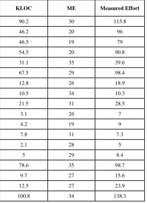
The NASA 18 software project dataset contains three parameters Kilo Line of Code (KLOC), Methodology (ME) and the Measured Effort for the 18 different software projects.
[image:2.595.315.545.493.685.2]
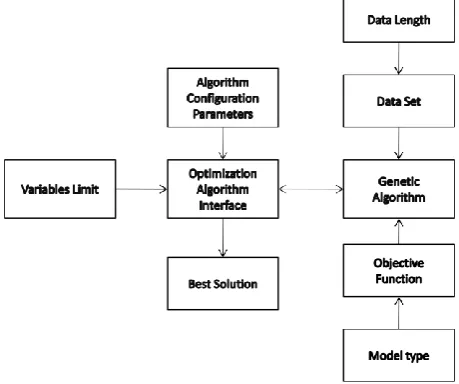
Fig 1: Block Diagram of the Simulated Model
Description of Block Diagram:
Algorithm Configuration Parameters- These parameters used in the simulation and according to the required performance their values have been set. As illustrated in table II.
Optimization Algorithm Interface- The variables limit and parameters are fed to this interface which is further applied in the GA. It receives the result of GA which is the best solution of our problem.
Data Length- It is the length of the population used for the simulation.
Data Set- In this research, we use NASA 18 data set to test.
Objective Function- The objective function for the problem is defined below in this section.
Model Type- Through the model type we select the model through which we want to optimize (i.e. model 1, 2 or 3).
Genetic Algorithm- This stage is to find optimal solution of software assessment. GA is chosen due to its ability in finding best possible solution as global search technique. The data length, data set, objective function and model type also acts as input to the genetic algorithm. The result of this stage is fed into the Optimization Algorithm Interface.
[image:3.595.308.548.112.314.2] Best Solution- As GA is a stochastic algorithm, we reach at a best solution after a number of iterations. The best solution is the optimal values of the measures used for assessment (i.e. the values of MMRE, MdMRE, MMER, PRED (25%), Time (sec)).
Table 1. NASA18 software project dataset
KLOC ME Measured Effort
90.2 30 115.8
46.2 20 96
46.5 19 79
54.5 20 90.8
31.1 35 39.6
67.5 29 98.4
12.8 26 18.9
10.5 34 10.3
21.5 31 28.5
3.1 26 7
4.2 19 9
7.8 31 7.3
2.1 28 5
5 29 8.4
78.6 35 98.7
9.7 27 15.6
12.5 27 23.9
100.8 34 138.3
[image:3.595.49.289.415.746.2]Following parameters are set for the simulation of the algorithm:
Table 2. Simulation Parameters
Parameters Name Value
amin 0
amax 10
bmin 0.3
bmax 2
cmin -0.5
cmax 0.5
dmin 0
dmax 20
Population size 16
Maximum generation 1000
The objective function for the problem is defined as:
Obj_fun = max{abs acteffor ti− esteffort i
acteffor ti
, = 1,2,3 … … 18}
Where,
actefforti = Actual Measured Effort ofith project.
estefforti = Estimated Effort of ith project on the basis of
selected values of a, b, c and d on respective formulas.
6.
SIMULATION RESULTS
The following measures are used to estimate the performances of the algorithm.
Magnitude of Relative Error (MRE): measures the error ratio between the actual effort and the predicted effort. It can be expressed as the following equation [10]:
MRE = actefforti − estefforti
actefforti
Magnitude of Error Relative to the estimate (MER): is given by [10]:
MER = actefforti − estefforti
estefforti
Mean Magnitude of Relative Error (MMRE):
MMRE = MREi
n i=1
n
Median Magnitude of Relative Error (MdMRE):
MdMRE = Median{MRE1, MRE2, … , MREn}
MMER = MERi
n i=1
n
PRED (25): This can be defined as the percentage of predictions falling within 25% of the actual values [10]:
PRED 25 = 1 ifMREi≤ 25 100 0 otherwise
n
[image:4.595.316.545.72.204.2]i=1
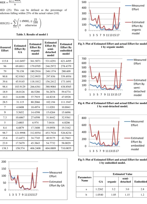
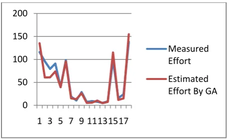
Table 3. Results of model 1
Measured Effort
Estimated Effort By
GA
Estimated Effort By organic
model
Estimated Effort By
semi-detached
model
Estimated Effort By embedded model
115.8 141.0497 361.5071 531.6291 621.4495 96 69.6811 179.0705 246.2972 278.4379 79 70.158 180.2916 248.1374 280.609 90.8 82.9363 212.9935 297.836 339.4954 39.6 45.9145 118.1812 156.2412 173.1691 98.4 103.9129 266.6361 380.9084 438.8565 18.9 18.0126 46.5286 56.2876 59.6774 10.3 14.6188 37.7919 44.8218 47.0528 28.5 31.115 80.2066 102.194 111.1947
7 4.0408 10.4974 11.0201 10.8841
9 5.5652 14.4398 15.6264 15.6696
7.3 10.6867 27.6598 31.8442 32.9361
5 2.6803 6.974 7.0416 6.8206
[image:4.595.62.541.76.742.2]8.4 6.6879 17.3408 19.0958 19.3162 98.7 121.9998 312.8554 453.7924 526.8234 15.6 13.4473 34.7745 40.9175 42.7843 23.9 17.5679 45.3843 54.7732 58.0029 138.3 158.574 406.2408 604.0889 710.0855
[image:4.595.51.299.154.727.2]Fig 2: Plot of Estimated Effort and actual Effort for model 1 by genetic algorithm.
[image:4.595.314.550.255.401.2]Fig 3: Plot of Estimated Effort and actual Effort for model 1 by organic model.
Fig 4: Plot of Estimated Effort and actual Effort for model 1 by semi-detached model.
Fig 5: Plot of Estimated Effort and actual Effort for model 1 by embedded model.
Parameters Name
Estimated Value
GA organic
semi-detached Embedded
a 1.2262 3.2 3.0 2.8
b 1.0540 1.05 1.15 1.2
0 50 100 150 200
1 3 5 7 9 11131517
Measured Effort
Estimated Effort By GA
0 100 200 300 400 500
1 3 5 7 9 11 13 15 17
Measured Effort
Estimated Effort By organic model
0 100 200 300 400 500 600 700
1 3 5 7 9 11 13 15 17
Measured Effort
Estimated Effort By semi-detached model
0 200 400 600 800
1 3 5 7 9 11131517
Measured Effort
[image:4.595.313.543.433.586.2]Measurement
Measurement Value
GA Organic
semi-detached Embedded
MMRE 23.2549 149.1211 219.6914 250.7279 MdMRE 21.0934 140.3788 221.055 264.5474 MMER 27.9117 56.4131 64.214 66.1623
Pred(25%) 61.1111 0 0 0
[image:5.595.49.284.228.742.2]Time(sec) 0.85158 1.7849 3.1236 3.1236
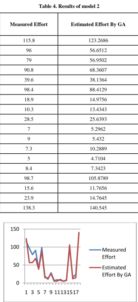
Table 4. Results of model 2
Measured Effort Estimated Effort By GA
115.8 123.2686
96 56.6512
79 56.9502
90.8 68.3607
39.6 38.1364
98.4 88.4129
18.9 14.9756
10.3 13.4343
28.5 25.6393
7 5.2962
9 5.432
7.3 10.2889
5 4.7104
8.4 7.3423
98.7 105.8789
15.6 11.7656
23.9 14.7645
138.3 140.545
Fig 6: Plot of Estimated Effort and actual Effort for model 2 by genetic algorithm.
Parameters Name Estimated Value By GA
a 0.58478
b 1.1821
c 0.11803
Measurement Measurement Value GA
MMRE 20.5639
MdMRE 22.5518
MMER 26.2881
Pred(25%) 66.6667
Time(sec) 0.82236
Table 5. Results of model 3
Measured Effort Estimated Effort By GA
115.8 135.1201
96 60.5491
79 60.9362
90.8 73.5736
39.6 39.397
98.4 95.5657
18.9 15.1244
10.3 13.1467
28.5 26.135
7 5.2912
9 5.7102
7.3 10.062
5 4.6484
8.4 7.1826
98.7 114.9918
15.6 11.7552
23.9 14.8567
138.3 154.6962
0 50 100 150
1 3 5 7 9 11131517
Measured Effort
Fig 7: Plot of Estimated Effort and actual Effort for model 3 by genetic algorithm.
Parameters Name Estimated Value GA
a 0.51764
b 1.2302
c 0.074869
d 1.2626
Measurement Measurement Value GA
MMRE 20.3292
MdMRE 19.4742
MMER 24.7371
Pred(25%) 72.2222
Time(sec) 0.83633
7.
CONCLUSION
Software parameter optimization is both crucial and important. In this paper the genetic algorithm (GA) is presented for the assessment of parameters of the proposed models (i.e. model 1, model 2 and model 3) for NASA software project dataset. The developed software assessment model based GA was capable of providing good assessment parameter optimization as compared to other known basic
models in the literature such as Organic model, Semi-detached model and Embedded model. The result shows that the three models(Organic model, Semi-detached model and Embedded model) takes much larger time and performs inferior than GA for the model1. In future the proposed models can be utilized for optimization using techniques such as swarm intelligence etc.
8.
REFERENCES
[1] Efi Papatheocharous, Harris Papadopoulos and Andreas S. Andreou. 2010. „Software Effort Estimation with Ridge Regression and Evolutionary Attribute Selection”, 3d Artificial Intelligence Techniques in Software Engineering Workshop, Larnaca, Cyprus.
[2] Alaa F. Sheta, Alaa Al-Afeef, “A GP Effort Estimation Model Utilizing Line of Code and Methodology for NASA Software Projects”, 10th International Conference on Intelligent Systems Design and Applications 978-1-4244-8136-1/10/2010.
[3] Alaa F. Sheta “Estimation of the COCOMO Model Parameters Using Genetic Algorithms for NASA Software Projects”, Journal of Computer Science 2 (2): 118-123, 2006.
[4] Kristin Bort and Monika Nerland “Software Effort Estimation as Collective Accomplishment”, Scandinavian Journal of Information Systems, 22(2), 65– 98, 2010.
[5] Iman Attarzadeh and Siew Hock Ow “Software Development Effort Estimation Based on a New Fuzzy Logic Model”, International Journal of Computer Theory and Engineering, Vol. 1, No. 4, 1793-8201,October2009. [6] Saleem Basha and Dhavachelvan P “Analysis of
Empirical Software Effort Estimation Models”, (IJCSIS) International Journal of Computer Science and Information Security, Vol. 7, No. 3, 2010.
[7] Randy K. Smith “Effort Estimation in Component-Based Software Development Identifying Parameters”, http://www.cs.utexas.edu/users/csed/doc_consortium/DC 98/smith.pdf.
[8] Barry Boehm. Software Engineering Economics. Englewood Cliffs, NJ:Prentice-Hall, 1981. ISBN 0-13-822122-7.
[9] Kemere, C.F., 1987. An empirical validation of software cost estimation models. Communication ACM, 30: 416-429.
[10] Ekrem Kocaguneli, Tim Menzies, and Jacky Keung “On the Value of Ensemble Effort Estimation”, Journal of IEEE Transactions on Software Engineering, Vol. X, 2012.
[11] Archive-be.com/pespmc1.vub.ac.be/GENETALG.html. 0
50 100 150 200
1 3 5 7 9 11131517
Measured Effort