Support vector machines for quality control of DNA sequencing

(1)

R E S E A R C H

Open Access

Support vector machines for quality control

of DNA sequencing

Ersoy Öz

1*

_{and Hüseyin Kaya}

2

*_{Correspondence:}

[email protected]

1_{Vocational School, Yildiz Technical}

University, Istanbul, Turkey Full list of author information is available at the end of the article

Abstract

Background:Support vector machines, one of the non-parametric controlled classifiers, is a two-class classification method introduced in the context of statistical learning theory and structural risk minimization. Support vector machines are basically divided into two groups as linear support vector machines and nonlinear support vector machines. Nonlinear support vector machines are designed to make classifications by creating a plane in a space by mapping data to that higher dimensional input space. This method basically involves solving a quadratic programming problem. In this study, the support vector machines, which have an increasing rate of use in pattern recognition area, are used in the quality control of DNA sequencing data. Consequently, the classification of quality of all the DNA sequencing data will automatically be made as ‘high quality/low quality’.

Results:The proposed method is tested against a dataset created from public DNA sequences provided by InSNP. We ﬁrst transformed all DNA chromatograms into feature vectors. An optimal hyperplane is ﬁrst determined by applying SVM to the training dataset. The instances in the testing dataset are then labeled by using the hyperplane. Finally, the estimated class labels are compared against the true labels by computing a confusion matrix. As the confusion matrix reveals, our method

successfully determines the labels of 23 out of 24 chromatograms.

Conclusions:We devised a new method to fulﬁll the quality screening of DNA chromatograms. It is a composition of feature extraction and support vector machines. It has been tested on a public dataset and it provided quite satisfactory results. We believe that it is a strong solution for DNA sequencing institutions to be used in automatic quality labeling of DNA chromatograms.

Introduction

Life sciences is one of the most demanding disciplines requiring advanced pattern recog-nition algorithms like clustering and classification techniques that are frequently used in molecular genetics and bioinformatics studies [, ]. With the advent of new DNA se-quencing techniques in the last two decades, the amount of data used in classification tasks has grown exponentially []. One of the main tasks in DNA sequencing centers is to classify the quality of DNA sequencing data [–]. Regarding this problem, a quality of DNA data, which is indeed a four-channel time series, needs to be classified as high or low quality. It is a critically important service especially for large DNA sequencing institutions since they need to know in advance before doing further analysis on data. It is also not a good practice to service low quality data to the customers. If the quality of data is known to be low, data might be reproduced by repeating necessary reactions. Manual labeling is

(2)

prohibitive or, in most cases, impossible because of large data size. It also requires human intervention which is sometimes error prone. Therefore automatic screening tools need to be devised.

In order to estimate the quality of DNA data, the classification method of support vec-tor machines (SVM), whose aim is to find an optimal hyperplane separating two different classes, can be used. It was first developed by Vapnik in  []. It is applied to tremen-dous number of diverse application fields like finance, telecommunication, life sciences and others [–]. Deterministic approach, strong mathematical ground, widely available software implementations and ease of use are the key factors of its success [].

Our aim in this article is to verify that SVM can be used as a powerful classification tech-nique to classify the quality of DNA chromatograms. In order to show this, we prepared a dataset consisting of publicly available DNA chromatograms []. We then manually de-termined the quality of each chromatogram in the dataset with the help of a bioinformatics expert. We also divided the dataset into training and testing []. We then transformed the chromatograms into a suitable format for SVM by extracting a set of feature vectors []. The next thing was the learning phase in which SVM was trained to find an optimal hy-perplane. Finally, we classified each data in testing dataset according to the trained SVM classifier. We measured the performance of the method by calculating a confusion matrix. The next two sections are reserved for explaining SVM and its variant in brief. In the fourth section, we explained the details of our approach in four steps: dataset preparation, feature extraction, training and testing. The article finishes with a conclusion.

Linear support vector machines

Linear support vector machines (LSVM) try to ﬁnd an optimum hyperplane which has the maximum margin among an inﬁnite number of hyperplanes separating the instances in the input space.

Linearly separable case

LetXdenote the training set consisting ofnsamples

X=(x,y), . . . , (xn,yn),xi∈Rd,yi∈ {–, +}

, ()

wherexiandyiare the sets of input vectors and corresponding labels, respectively [].

The decision function issignum(f(x)), wheref(x) is the discriminant function associated with the hyperplane and deﬁned as

f(x) =wTxi+b, w∈Rdandb∈R. ()

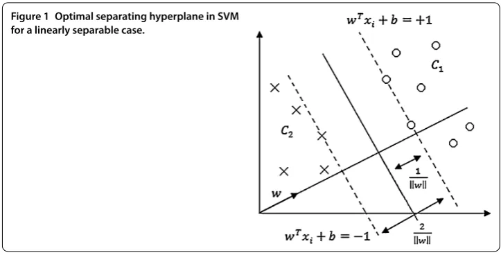
Our aim here is to determine the vector wand the scalarbwhich together deﬁne the optimum hyperplane shown in Figure . The hyperplane should satisfy the following con-straints:

wTxi+b≥+ foryi= +, ()

(3)

[image:3.595.116.478.81.265.2]

Figure 1 Optimal separating hyperplane in SVM for a linearly separable case.

These constraints can be written in a single form with little eﬀort

yi

wTxi+b

≥+, i= , . . . ,n. ()

A margin band is deﬁned as the region between hyperplanes wTxi +b = + and

wT_x

i+b= – []. The width of the margin band can easily be calculated as /w. For the

separable case, a maximum margin band can be determined by minimizing the inverse of the distance as in the following quadratic optimization problem with linear constraints:

Object function: min/w, ()

Subject to:yi

wTxi+b

≥+, i= , . . . ,n. ()

It is proved that an optimal hyperplane exists and is unique so that the negative instances lie on one side of the hyperplane and the positive instances lie on the other []. The opti-mization problem in Eq.  can be formulated as an unconstrained optiopti-mization problem by introducing Lagrange multipliers:

Lp= /w– n

i=

αi

yi

wTxi+b

– , ()

whereαiare Lagrange multipliers. The Lagrangian functionLphas to be minimized with

respect towandband maximized with respect toαi≥. By using Karush-Kuhn-Tucker

(KKT) conditions, the design variableswandbin Eq.  can be expressed in terms ofαi,

which then transforms the problem into a dual problem that requires only maximization with respect to the Lagrangian multipliersαi

∂Lp

∂w = →

n

i=

αiyixi=w, ()

∂Lp

∂b = →

n

i=

(4)

The dual problem is constructed by substituting Eq.  and Eq.  into Eq. , from which the dual form of a quadratic programming (QP) problem can be obtained as follows:

Ld= n

i=

αi– / n

i=

n

j=

αiαjyiyjxTixj. ()

Then we solve the dual problem with respect toαiand subject to the constraints

n

i=

αiyi=  and αi≥. ()

This QP problem is then solved by any standard quadratic optimization method to de-termineαi. Although there are nsuch variables, most of them vanish. The instancesxi

corresponding to positiveαivalues are called support vectors. Finally, the vectorwis

de-termined by using Eq. . The last unknown parameterbis determined by taking average of

b=yi–wTxi ()

for all support vectors [].

Linearly nonseparable case

In the previous section, we assumed that the data can be perfectly separable in the sense that the data samples of different class labels resides on different regions. However, in prac-tice, such a hyperplane may not be found because of the specific distribution of instances in the data. This makes linear separability difficult as the basic linear decision boundaries are often not sufficient to classify patterns with high accuracy.

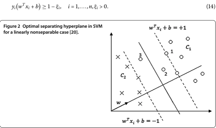
If the data is not separable, then the constraint in Eq.  may not hold. This corresponds to the data sample that falls within the margin or on the wrong side of the decision bound-ary as shown in Figure . In order to handle the nonseparable data, the formulation is generalized by introducing a slack variableξ for each instance

yi

wTxi+b

[image:4.595.118.478.520.734.2]

≥ –ξi, i= , . . . ,n,ξi> . ()

(5)

The new optimization problem is deﬁned as the combination of two goals: margin max-imization and error minmax-imization. Ifξi= , the instancesxiare correctly classiﬁed (the

point  in Figure ). When  <ξi< , the instancesxiare also correctly classiﬁed, but they

are inside the margin (the point  in Figure ). Finally,ξi≥, the instancesxiare wrongly

classiﬁed (the point  in Figure ). The number of misclassiﬁcations is the number ofξ

greater than . On the other hand, the number of nonseparable points is the number of positiveξi. Finally, the soft error is deﬁned as follows:

n

i=

ξi.

It is added also to the primal of Eq. :

Lp= /w+C n

i=

ξi– n

i=

αi

yi

wTxi+b

–  +ξi

–

n

i=

μiξi ()

ξivalues are guaranteed to be positive by the new Lagrange parametersμi. The parameter

C is used to set the weight between the number of support vectors and the number of nonseparable points. In other words, the instances inside the margin band are penalized together with the misclassiﬁed instances to reach a better generalization in testing.

The dual problem is

Ld= n

i=

αi– / n

i=

n

j=

αiαjyiyjxTixj ()

subject to

n

i=

αiyi= , and ≤αi≤C. ()

The methods in the separable case can be applied to the nonseparable case. The instances for whichαi=  hold are not support vectors. The remaining part of the equation that

deﬁnes the parameterswandbcan be determined similarly [].

Nonlinear support vector machines

When the data is nonlinearly separable, the linear SVM is not profitable. It is better to use a nonlinear SVM for this situation. In order to transform this input, the nonlinear SVM first uses a nonlinear kernel and then a linear SVM. The nonlinear kernel function, which most probably is a large matrix, makes the nonlinear SVM take a very long time when mapping the input to a higher dimensional space []. Here, the purpose is to find the separating hyperplane that has the highest margin in the new dimension, the one where the data are transformed.

To transform the nonlinearly separable data into linearly separable data, the data are mapped in the formφ:Rn_→_H_{using a nonlinear function}_φ_{into a higher dimensional}

(6)

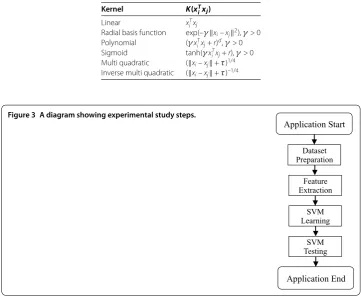
Table 1 The most typical kernel functions in the literature whereγ,r,τanddare kernel parameters

Kernel K(xT

ixj)

Linear xT

ixj

Radial basis function exp(–γxi–xj2),γ> 0

Polynomial (γxT

ixj+r)d,γ> 0

Sigmoid tanh(γxT

ixj+r),γ> 0

Multi quadratic (xi–xj+τ)1/4

[image:6.595.116.478.106.409.2]

Inverse multi quadratic (xi–xj+τ)–1/4

Figure 3 A diagram showing experimental study steps.

a linear classiﬁcation problem is formulated []. Depending on this, Eqs.  and , which point to the Lagrangian of the dual optimization problem, need to change as follows:

Ld= n

i=

αi– / n

i=

n

j=

αiαjyiyjK

xT_ixj

. ()

A kernel function is expressed as follows and it involves the input vectors:

KxT_i xj

=φ(xi)Tφ(xj). ()

The majority of theφ(·) transformations are not known. However, it is possible to get the dot product of the corresponding space using an input vector function [].

Kernel functions need to have a corresponding inner product in the feature space which is transformed. This is stated in Mercer’s theorem []. In this way, the solution of a dual problem gets simpler because there is no need to make calculations for the inner products in the transformed space. Commonly used kernels are shown in Table .

Application

(7)

[image:7.595.118.478.80.259.2]

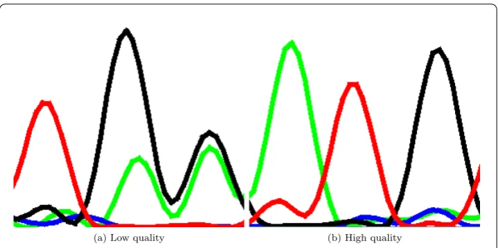
Figure 4 Sample regions from two DNA chromatograms.On the left, two peaks are overlapped whereas in the right ﬁgure, secondary peaks are much closer to the baseline.

Dataset

In order to evaluate the performance of the proposed method, a benchmark dataset should be available. To create the dataset, we selected  DNA chromatograms from InSNP database. The data in each chromatogram is a four-channel time series with diﬀerent lengths. Each channel is a series of Gaussian shaped peaks along the time axis which con-tains information about the nucleotides A, C, G and T, respectively.

We then manually screened each data and labeled the quality of a data as high if its peaks were well resolved. We labeled the quality of a data as low if its peaks were overlapped and had low signal to noise ratio. The example for such a case is shown in Figure . We followed SVM labeling convention and chose the labels – and + for high and low quality.

Feature extraction

We cannot give DNA chromatograms directly as input data to SVM. First of all, they have different lengths and are too long. Using whole length data is not a good strategy. So, we should create a set of features representing the statistical characteristics of each data. The number of features should be low and fixed. Also, the features should be chosen to best represent the quality of the chromatograms []. To fulfill these requirements, the following set of features are chosen:

. Average of all values in the data.

. Standard deviation of all values in the data. . Median of all values in the data.

. Average of all values created for each peak available in all of the four channels of the data.

. Standard deviation of all values created for each peak available in all of the four channels of the data.

. Median of all values created for each peak available in all of the four channels of the data.

. The number of peaks.

(8)

[image:8.595.234.362.94.163.2]

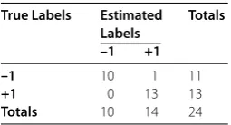
Table 2 Confusion matrix

True Labels Estimated Labels

Totals

–1 +1

–1 10 1 11

+1 0 13 13

Totals 10 14 24

Having determined the features, we processed each data and obtained a feature vector. Each feature vector is accompanied with a label determined in the previous step. In con-clusion, we converted the dataset of DNA chromatograms into an input matrix and output vector. From now on, the data is ready for SVM.

Training

SVM needs to be trained before making classification. So, we reserved some of the data for training by randomly selecting  data. We need to give a training set into SVM so that it can create a hyperplane. However, we must first adjust the parameters. The most important parameter isCin Eq. . We can setC=  if we are sure that the data is linearly separable. We know that it is generally not perfectly linearly separable. So, we giveC=  to make it flexible. SVM is then run for the training samples.

Testing

Now we have a hyperplane provided by SVM. We should use this hyperplane to classify other samples in the data usingsignum(f(x)). We used  of them in training, so the testing set has  samples. We run SVM for testing. A confusion matrix for SVM testing is pre-sented in Table . As indicated in the table, SVM correctly classiﬁes almost all instances in the testing set. There is only one mistake which is false positive. This is a very promising result. It means we can use SVM for automatic quality screening of DNA chromatograms.

Conclusion

We developed a new quality evaluation technique in which the quality of a DNA chro-matogram is classiﬁed as low or high. In this sense, it is a two-class classiﬁcation problem for which SVM is chosen. To apply SVM, some sets of features of the chromatograms are extracted. SVM is trained on a training set to learn the hyperplane; SVM is then run on the testing set, from which a confusion matrix is created. As it clearly shows, the results are quite satisfactory as only one mistake was made. Therefore, our method is a good solution for automatic screening of DNA data, especially for large DNA sequencing facilities.

Competing interests

The authors declare that they have no competing interests.

Authors’ contributions

HK conceived of the study and participated in its design and coordination. EO participated in the implementation and classiﬁcation. EO drafted the manuscript. All authors read and approved the ﬁnal manuscript.

Author details

1_{Vocational School, Yildiz Technical University, Istanbul, Turkey.}2_{Informatics Institute, Istanbul Technical University,}

Istanbul, Turkey.

Acknowledgements

Dedicated to Professor Hari M Srivastava.

(9)

References

1. Furey, T, Cristianini, N, Duﬀy, N, Bednarski, D, Schummer, M, Haussler, D: Support vector machine classiﬁcation and validation of cancer tissue samples using microarray expression data. Bioinformatics16(10), 906-914 (2000) 2. Mateos, A, Dopazo, J, Jansen, R, Tu, Y, Gerstein, M, Stolovitzky, G: Systematic learning of gene functional classes from

DNA array expression data by using multilayer perceptrons. Genome Res.12(11), 1703-1715 (2002) 3. Lander, E, et al.: Initial sequencing and analysis of the human genome. Nature409(6822), 860-921 (2001) 4. Ewing, B, Hillier, L, Wendl, M, Green, P: Base-calling of automated sequencer traces using Phred. I. Accuracy

assessment. Genome Res.8(3), 175-185 (1998)

5. Chou, HH, Holmes, MH: DNA sequence quality trimming and vector removal. Bioinformatics17(12), 1093-1104 (2001). http://bioinformatics.oxfordjournals.org/content/17/12/1093.abstract

6. Otto, TD, Vasconcellos, EA, Gomes, LHF, Moreira, AS, Degrave, WM, Mendonca-Lima, L, Alves-Ferreira, M: ChromaPipe: a pipeline for analysis, quality control and management for a DNA sequencing facility. Genet. Mol. Res.7(3), 861-871 (2008). (3rd International Conference of the Brazilian-Association-for-Bioinformatics-and-Computational-Biology, Sao Paulo, BRAZIL, NOV 01-03, 2007)

7. Cortes, C, Vapnik, V: Support-vector networks. Mach. Learn.20(3), 273-297 (1995)

8. Guyon, I, Weston, J, Barnhill, S, Vapnik, V: Gene selection for cancer classiﬁcation using support vector machines. Mach. Learn.46(1-3), 389-422 (2002)

9. Bhardwaj, N, Langlois, R, Zhao, G, Lu, H: Kernel-based machine learning protocol for predicting DNA-binding proteins. Nucleic Acids Res.33(20), 6486-6493 (2005)

10. Brown, M, Grundy, W, Lin, D, Cristianini, N, Sugnet, C, Furey, T, Ares, M, Haussler, D: Knowledge-based analysis of microarray gene expression data by using support vector machines. Proc. Natl. Acad. Sci. USA97(1), 262-267 (2000) 11. Vercoutere, W, Winters-Hilt, S, Olsen, H, Deamer, D, Haussler, D, Akeson, M: Rapid discrimination among individual

DNA hairpin molecules at single-nucleotide resolution using an ion channel. Nat. Biotechnol.19(3), 248-252 (2001) 12. Ravi, V, Kurniawan, H, Thai, PNK, Kumar, PR: Soft computing system for bank performance prediction. Appl. Soft

Comput.8(1), 305-315 (2008)

13. Elish, KO, Elish, MO: Predicting defect-prone software modules using support vector machines. J. Syst. Softw.81(5), 649-660 (2008). (Joint Meeting of the International Workshop on Software Measurement (IWSM)/International Conference on Software Process and Product Measurement (MENSURA), Palma de Majorque, SPAIN, NOV 05-07, 2007)

14. Hearst, M: Support vector machines. IEEE Intell. Syst. Appl.13(4), 18-21 (1998)

15. Manaster, C, Zheng, W, Teuber, M, Wachter, S, Doring, F, Schreiber, S, Hampe, J: InSNP: a tool for automated detection and visualization of SNPs and InDels. Human Mutat.26(1), 11-19 (2005)

16. Jain, A, Duin, R, Mao, J: Statistical pattern recognition: a review. IEEE Trans. Pattern Anal. Mach. Intell.22(1), 4-37 (2000) 17. Sun, S, Zhang, C: Adaptive feature extraction for EEG signal classiﬁcation. Med. Biol. Eng. Comput.44(10), 931-935

(2006)

18. Campbell, C, Ying, Y: Learning with Support Vector Machines. Morgan & Claypool Publishers, San Rafael (2011) 19. Vapnik, VN: Statistical Learning Theory. Wiley, New York (1998)

20. Alpaydin, E: Introduction to Machine Learning. MIT Press, Cambridge (2004)

21. Yue, S, Li, P, Hao, P: SVM classiﬁcation: its contents and challenges, applied mathematics. Appl. Math. J. Chin. Univ. Ser. B18(3), 332-342 (2003)

22. Cherkassky, V, Mulier, FM: Learning from Data: Concepts, Theory, and Methods. Wiley-Interscience, New York (1998) 23. Martínez-Ramon, M, Cristodoulou, C: Support Vector Machines for Antenna Array Processing and Electromagnetics.

Morgan & Claypool Publishers, San Rafael (2006)

24. Scholkopf, B, Smola, A: Learning with Kernels. MIT Press, Cambridge (2001)

25. Chang, CC, Lin, CJ: LIBSVM: a library for support vector machines. ACM Trans. Intell. Syst. Technol.2(3), Article ID 27 (2011). (Software available at http://www.csie.ntu.edu.tw/~cjlin/libsvm)

26. Andrade-Cetto, L, Manolakos, E: Feature extraction for DNA base-calling using NNLS. In: Statistical Signal Processing, 2005 IEEE/SP 13th Workshop on, pp. 1408-1413 (2005)

doi:10.1186/1029-242X-2013-85