An accelerated and accurate three dimensional ray tracing using red black tree with facet mining and object bouncing techniques

c

T ¨UB˙ITAK

doi:10.3906/elk-1212-98 h t t p : / / j o u r n a l s . t u b i t a k . g o v . t r / e l e k t r i k /

Research Article

An accelerated and accurate three-dimensional ray tracing using red-black tree

with facet mining and object bouncing techniques

Mohammad Jakirul ISLAM1_{, Ahmed Wasif REZA}1,∗, Kamarul Ariffin NOORDIN1, Kaharudin DIMYATI2_{, Abu Sulaiman Mohammad Zahid KAUSAR}1

1_{Department of Electrical Engineering, Faculty of Engineering, University of Malaya, Kuala Lumpur, Malaysia} 2_{Faculty of Engineering, National Defence University of Malaysia, Kuala Lumpur, Malaysia}

Received: 19.12.2012 • Accepted: 18.04.2013 • Published Online: 23.02.2015 • Printed: 20.03.2015

Abstract: Recent trends show that it is a major challenge to predict the exact propagation path accurately and efficiently for three-dimensional (3D) indoor environments. Therefore, this study introduces a new 3D ray tracing algorithm based on a red-black tree with facet mining and object bouncing techniques. The red-black tree data structure offers a faster object searching operation while repeatedly performing intersection tests. On the other hand, extensive ray-facet intersection tests can be eliminated by using object and facet bouncing techniques, whereas the facet mining makes it easier to trace the transmitted ray paths accurately. The proposed method is compared with ray launching, bidirectional path tracing, modified angular Z-buffer, and binary space partitioning-based modified wavefront decomposition techniques and it is found that it obtains better prediction results in terms of computation time, the number of predicted rays, and radio propagation path loss.

Key words:Ray tracing, red-black tree, facet mining, object bouncing

1. Introduction

The root of the wireless communication is the propagation of radio waves. Comprehensive understanding and appropriate characterization of radio wave propagation can only make easier the optimal deployment of indoor wireless networks. Hence, modeling of radio wave propagation prediction has been an attractive research area for many years. Moreover, data transmission through a wireless device in indoor locations has also been gaining popularity in recent years and has led to the use of small coverage areas, higher frequency bands, and higher data rates, making propagation prediction more challenging. Ray tracing [1] is a widely used technique to predict the propagation paths in indoor environments. Predicting the rays requires extremely accurate information about the objects of the realistic environments. On the other hand, calculations of ray paths can be computationally expensive due to the large number of rays that must be traced.

For the characterization of radio wave propagation, many two-dimensional (2D) ray tracing models [2–4] are found in the literature. Basically, 2D models are faster but less accurate compared to the three-dimensional (3D) method because 2D models only trace the fewer rays that are propagated through the horizontal direction. On the other hand, 3D models are slower but provide better ray prediction accuracy, because they can trace all the rays that are propagated in any direction. In order to overcome the drawbacks of the 2D model, a number of 3D ray tracing methods have already been developed. Most of them are based on image [5–7],

bouncing-ray (SBR) [8,9], bidirectional path tracing (BDPT) [10], ray launching (RL) [11], angular Z-buffer (AZB) [12], and modified angular Z-buffer (MAZB) [13] techniques. The image method is precise but suffers from inefficiency when the number of objects involved is relatively larger. Hence, its use is restricted to simple environments. The RL technique is applicable to complex environments but it also suffers from inefficiency. In the SBR technique, ray tubes are used to cover the spherical wavefront at the receiving location. If a receiver (Rx) is located in the overlapping area between the ray tubes, Rx will then receive two rays and hence a ray double-counting error will occur. To overcome these disadvantages and accelerate the ray tracing, the modified wavefront decomposition (MWD) method was introduced in [14]. In MWD, the binary space partitioning (BSP) technique is used for the acceleration of the ray tracing method. However, a BSP tree withS number of facets needsO(S) time for the worst-case condition and O(SlogS) time for the best-case condition while performing an intersection test, which are still large enough. On the other hand, BDPT offers inaccurate ray prediction results in some circumstances and fails to decrease the computational time due to double ray tracing and a great amount of intersection tests. Another accelerated ray tracing based on MAZB was presented in [13]. According to this algorithm, the simulation space is divided into a number of angular regions and it stores each facet of the environment in the regions of the array where they belong. Afterwards, for each ray, only the objects of a particular region take part in ray-facets intersection tests. However, it is necessary to distribute the S number of facets among the circular regions and it wastes O(S) time. After that, a search operation is made to identify the particular region among the Xregions, which will take another O(X) time. Therefore, O(SX) time is

needed prior to the intersection time, whereas O(S′) time is needed for a single intersection test, where S′ is the number of facets existing in a particular angular region. Moreover, this method is not suitable for multiple reflections, because there are many source points and an AZB is needed to be built for each of them [3].

Therefore, this study has developed an accelerated and accurate 3D ray tracing algorithm, namely red-black tree with facet mining and object bouncing (RBTreeFMOB), that will overcome the limitations of the existing ray tracing techniques as stated before. The facet mining technique is introduced here so that the processing time of unnecessary facets is minimized during the intersection test, and an exact and accurate intersection point on a facet can easily be found during the ray tracing. Conversely, a better ray prediction time is achieved by the red-black tree (RBTree) along with the object and facet bouncing techniques. The superiority of the proposed RBTreeFMOB algorithm will be proved in terms of ray prediction accuracy, computational efficiency, and path loss accuracy by comparing it with the existing ray tracing techniques.

2. Ray tracing procedure

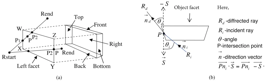
For the simulation, objects are created by 3D cube or cuboids in a 3D coordinate system, as illustrated in Figure 1. The proposed algorithm uses a balanced binary tree, namely RBTree, to reduce the ray-facet intersection time. The searching operation consumes a computational time of O(logN) because the RBTree always has a depth of O(logN) , where N is the number of objects [15]. In this study, the RBTree is used to store the 3D objects and is constructed according to the object ID, as presented in Figure 1.

Figure 2a. Similarly, for the second quadrant, the right/bottom facet is taken out of the 3D object. Top/bottom and top/left facets are needed to be taken out of the 3D object in the case of the third and fourth quadrant, respectively. 1 2 4 8 6 3 5 7 12 10

9 11 13

12 15 16 Root node Black node Red node

Figure 1. Illustration of a simple 3D indoor environment and corresponding RBTree made from the objects of this environment. (b) (a) Rstart Rend Rend P2 P

P1 P P2

W

X

Y

Left facet Back Bottom

Front Top Right d

θ

θ

R

S

−

S

n

n

R

Object facet Here,

d

R

i

R

θ

P-intersection point →

n

S

Pn

S

Pn

⋅

=

−

⋅

P

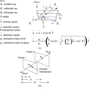
Figure 2. (a) Facet mining and identification of intersection point; (b) diffraction of a ray.

(a) (b) Rstart Rend Facet 1 Facet 2 P P’ d d’ d” Closest Intersection i θ r R → S i n → r n → i R Object 1 P r θ t θ 2 P t n → R_t

1 2 η η Here, i

R_{-incident ray}

r

R _{-reflected ray}

t

R_{-refracted ray}

θ-angle

→

S-normal vector

→

n-direction vector P-intersection point

→

n-ditrection vector

1

η -refractive index of air

2

η -refractive index of glass

→ →

→

−

=n S

n

i i

r 2cosθ

(

)

= n S

n i i i t θ η η θ η η η η 2 2 2 1 2 1 2

1 _{cos 1 1 cos}

(

( )

)

Figure 3. (a) Reflection, refraction, and transmission of a ray; (b) determination of the closest intersection point based on the distance from the ray’s emanating point.

However, if the ray intersects more than one object, then the closest intersection point (shown in Figure 3b) is identified based on the distance from the ray’s origin point. According to Figure 3(b), the intersection

point P is the closest intersection point, because P is closer than point P′ in respect to the origin of the emanated ray.

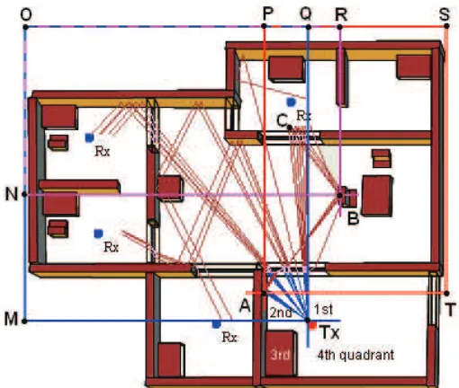
Details about the ray tracing procedure are described as follows. Referring to Figure 4, after launching a ray T xA from the origin ofTx, an intersection test is intended to identify the closest intersection point A. For this, first, we have to calculate the quadrant of the launched ray, followed by splitting the whole space into four different quadrants at the origin of that ray. A rectangleTxMOQ is required to be formed in the second quadrant because the ray T xA traveled in the second quadrant. Only the objects in the second quadrant (inside rectangleTxMOQ), ignoring the three other quadrants, will be searched within the RBTree to identify the closest intersection point A. By simple containment test of start and end coordinates of each 3D object, we can determine on which quadrant (rectangle) the object lies. Let the coordinates of test point be P(xp, yp),

and the rectangle’s upper left point is P₁(x₁, y₁) and the lower right point is P₂(x₂, y₂) . If xp is between x1

and x₂, and yp is between y1 and y2, then the test point P(xp, yp) is inside the rectangle. The ray AB will

Figure 4. Illustration of significant predicted rays and object bouncing technique for 3D indoor environment.

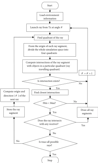
This procedure will continue until a ray segment hits any receiver or passes away from the indoor environment. For instance, ray segment BC hits the receiver, and therefore the signal path T xC (which is composed of connected line segments T xA, AB, andBC) is considered as a significant signal path. Once the receiver receives a ray, another ray is needed to be launched from the position of T x. The overall flowchart of the proposed method is given in Figure 5.

From the above discussions, we may conclude that, for each ray segment, an intersection test will be done with the objects that lie in a particular quadrant and the rest will be bounced. Moreover, the facet bouncing technique is capable of overlooking the unnecessary object facet, which can further minimize the significant amount of intersection tests of the proposed ray tracing method. Finally, a huge amount of computational time can be reduced by using the object and facet bouncing techniques.

If on average S′ _{number of object facets participate in the intersection test, then the complexity of a}

single intersection test isO(logS′) for the proposed RBTreeFMOB algorithm. For m number of launched rays, a comparison of time complexity between the existing techniques and the proposed RBTreeFMOB algorithm is projected in the Table.

Table. Time complexity of different algorithms.

Algorithm Ray launching time Average intersection time Complexity

BDPT [10] O(m) O(S2_{) O(mS}2₎

RL [11] O(m) O(S) S_×O(mS)

MAZB [13] O(m) O(S′+SX) O(m(S′+SX))

MWD [14] O(m) O(SlogS) O(mSlogS)

RBTreeFMOB O(m) O(logS′) O(mlogS′)

less computational time compared to the BDPT [10] and RL [11] methods because, after distribution of the facets among the angular regions, fewer facets are taking part in each intersection test in the MAZB technique. Moreover, the MWD method used a BSP tree to accelerate the ray tracing, whose best-case complexity follows the logarithmic time instead of linear search time.

Compute origin and direction ( θ ) of the

next ray

Start

Launch ray from Tx at angle θ

Find quadrant of the ray

From the origin of each ray segment, divide the whole simulation space into

four quadrants

Compute intersections of the ray segment with objects in a particular quadrant (ray

travelling quadrant)

Is intersection exists?

Find closest intersection

Hits < Max?

Does the ray intersects with any receiver? Load environment

information

Is trace all possible rays?

Draw all ray segments

1 + = θ θ

Stop Store the ray

segment

Yes

Yes

Yes

Yes

No

No

No No

3. Results

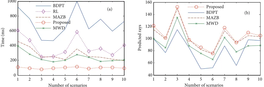
To perform a fair comparison between the algorithms, the proposed method has been implemented over C# Object Oriented Programming (OOP) and all settings were retained similarly. The results are taken from the indoor environment presented in Figure 4, where labels Tx and Rx represent the transmitter and receiver, respectively. The comparison figures are drawn from the simulation results obtained by placingTx in different locations while Rxis kept steady in the simulation environment of Figure 4. In order to predict the path loss, the permittivity of the brick walls and glass doors (as presented in Figure 4) are assumed to be 5.2 and 3.2, respectively. The height and thickness of the walls are 280 cm and 12.7 cm, respectively. During this simulation, a semispherical antenna is used for both the transmitting and receiving antenna and they are operated at 900 MHz carrier frequency. Moreover, the transmitter and receivers are placed at a height of about 140 cm from the ground. Figure 6a shows a comparison based on the computation times for different ray tracing algorithms.

2 4 6 8 10

1 3 5 7 9

0 200 400 600 800 1000

Number of scenarios

Time (ms)

BDPT RL MAZB Proposed MWD

(a)

2 4 6 8 10

1 3 5 7 9

40 60 80 100 120 140 160

Number of scenarios

Predicted rays

Proposed BDPT MAZB MWD

(b)

Figure 6. Comparison between the proposed and existing algorithms based on the (a) ray prediction time and (b) number of predicted rays.

It is observed that the proposed RBTreeFMOB algorithm gives higher computational efficiency compared to the BDPT [10], RL [11], MAZB [13], and MWD [14] methods, which are 73.98%, 85.62%, 64.44%, and 57.98% on average, respectively. It is obvious from Figure 6a that the obtained ray prediction time is fairly consistent for the given scenarios. Moreover, as ray prediction accuracy is the same with the RL technique, the proposed RBTreeFMOB algorithm provides better accuracy of about 22% (on average) than the BDPT, better accuracy of 3% than the MAZB, and better accuracy of 7% than the MWD techniques, respectively, as depicted in Figure 6b.

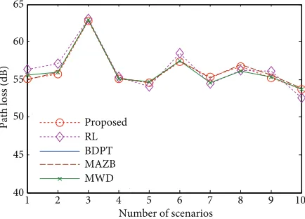
Additionally, a comparison based on the predicted path loss is illustrated in Figure 7. The indoor path loss can be calculated from the free space loss and loss obtained by the reflection, refraction, and diffraction of the rays that can be computed from [19].

between the proposed RBTreeFMOB algorithm and recent well-known accelerated algorithms such as MAZB and MWD.

2 4 6 8 10

1 3 5 7 9

40 45 50 55 60 65

Number of scenarios

Path

l

oss (dB)

Proposed RL BDPT MAZB MWD

Figure 7. Comparison between the proposed and existing algorithms based on the average path loss.

4. Conclusion

A new RBTreeFMOB algorithm is introduced in this study. To accelerate the proposed RBTreeFMOB al-gorithm, the RBTree along with the object and facet bouncing techniques are used, which perform a single

intersection with O(logS′) time instead of linear search time. Conversely, the facet mining technique provides the exact propagation path and offers better ray prediction accuracy than the existing algorithms. The predicted results confirm that the RBTreeFMOB algorithm achieves better ray prediction time and better ray prediction accuracy as well as provides a well-matched path loss curve when compared to the RL, BDPT, MAZB, and MWD methods. The proposed algorithm will facilitate wireless radio networks and personal communication systems inside buildings.

References

[1] Sarker MS, Reza AW, Dimyati K. A novel ray-tracing technique for indoor radio signal prediction. J Electromagnet Wave 2011; 25: 1179–1190.

[2] Mart´ınez D, Las-Heras F, Ayestaran RG. Fast methods for evaluating the electric field level in 2D-indoor environ-ments. Prog Electromagn Res 2007; 69: 247–255.

[3] Iskander MF, Yun AZ. Propagation prediction models for wireless communication systems. IEEE T Microw Theory 2002; 50: 662–673.

[4] Yang M, Stavrou S, Brown AK. Hybrid ray-tracing model for radio wave propagation through periodic building structures. IET Microw Antenna P 2011; 5: 340–348.

[5] Tiberi G, Bertini S, Monorchio A, Giannetti F, Manara G. Computationally efficient ray-tracing technique for modelling ultrawideband indoor propagation channels. IEEE Antenn Propag M 2009; 57: 395–401.

[6] Liu ZY, Guo LX. A quasi three-dimensional ray tracing method based on the virtual source tree in urban micro-cellular environments. Prog Electromagn Res 2011; 118: 397–414.

[7] Maltsev A, Maslennikov R, Lomayev A, Sevastyanov A, Khoryaev A. Statistical channel model for 60 GHz WLAN systems in conference room environment. Radioengineering 2011; 20: 409–422.

[9] Jianjun D, Ru-Shan C, Huan Z, Fan ZH. An improvement for the acceleration technique based on monostatic bistatic equivalence for shooting and bouncing ray method. Microw Opt Techn Lett 2011; 53: 1178–1183.

[10] Cocheril Y, Vauzelle R. A new ray-tracing based wave propagation model including rough surfaces scattering. Prog Electromagn Res 2007; 75: 357–381.

[11] Raida Z, Lukes Z, Lacik J. On using ray-launching method for modeling rotational spectrometer. Radioengineering 2008; 17: 98–107.

[12] de Adana SF, Gutierrez Blanco O, Diego IG, Perez Arriaga J, Catedra MF. Propagation model based on ray tracing for the design of personal communication systems in indoor environments. IEEE T Veh Technol 2000; 49: 2105–2112.

[13] Saeidi C, Hodjatkashani F. Modified angular Z-Buffer as an acceleration technique for ray tracing. IEEE T Antenn Propag 2010; 58: 1822–1825.

[14] Mohtashami V, Shishegar AA. Modified wavefront decomposition method for fast and accurate ray-tracing simula-tion. IET Microw Antenna P 2012; 4: 295–304.

[15] Cormen TH, Leiserson CE, Rivest RL, Stein C. Introduction to Algorithms. 3rd ed. Cambridge, MA, USA: MIT Press, 2009.

[16] Gatland IR. Thin lens ray tracing. Am J Phys 2002; 70: 1184.

[17] Smith CJ. A Degree Physics. Part III, Optics. London, UK: Edward Arnold Publishers, 1960.

[18] Tsingos N, Funkhouser T, Ngan A, Carlbom I. Modelling acoustics in virtual environments using the uniform theory of diffraction. In: Proceedings of the 28th Annual Conference on Computer Graphics and Interactive Techniques. New York, NY, USA: ACM, 2001. pp. 545–552.