Journal of Chemical and Pharmaceutical Research, 2016, 8(7):651-666
Research Article
CODEN(USA) : JCPRC5
ISSN : 0975-7384
Analytical Solutions of SIRS-SI Malaria Disease Model Using HPM
R. Senthamarai and S. Balamuralitharan
Department of Mathematics, SRM University, Kattankulathur-603 203, Tamil Nadu, India
ABSTRACT
In this paper, we discussed the transmission of malaria disease in the work of an SIRS-SI model with treatments are given to humans and mosquitoes. Furthermore, we investigated the Homotopy Perturbation Method (HPM) to construct the approximate analytical solution of the simultaneous non linear ordinary differential equations arise in this model. A stability analysis was then performed and MATLAB numerical simulation was provided to clarify the result. These analytical solutions represent a significant simplification of the system’s description allowing easy curve fitting to experiment. Analytical results are compared with simulation results and satisfactory agreement is noted.
Key words: HPM, Malaria Disease, SIRS-SI model.
INTRODUCTION
The general epidemic model with some effective features is described in [1, 2]. The epidemiological impact of immunity to malaria has been investigated in [3, 4]. The effect of vaccines for malaria has been investigated in [5]. The disease modification idea has been discussed in [5]. However the intensity of malaria transmission changes over the evolution of drug resistance is explained in [6]. In [7], the different fluctuation of the mosquito density is investigated. In [8], the authors considered the treatment and vaccination strategies on the transmission of malaria. A mathematical model for malaria treatment and drug resistance is described in [9]. A model interaction with constant immigration in human population and infective immigrants has been depicted in [10].
The dynamics of a malaria transmission model in environment is dealt in [11]. The Modelling of malaria transmission by considering the human population is exhibited in [12], where it is assumed that the individuals recovered from malaria can act as infectives for susceptibles mosquitoes. The idea of reservoir class is also incorporated in [13]. This method of control is cheap and is being used in many part of the area. But the disease is endemic. The larvivorous fish to control malaria by decreasing the larvae population is developed in [14]. The optimal control approach is used to minimize the infectives rate of mosquito. The paper [15] discussed on the study of optimal control on vaccination program. In this paper, we formulated a non-linear differential equations model by malaria transmission. We found the HPM and analyzed the stability of this equilibrium [16-22].
NOMENCLATURE ℎ Susceptible human ℎ Infected human
ℎ Recovered human,
Susceptible mosquito Infected mosquito
ℎ rate of constant
1 rate of blood transfusion 2 rate of infected mosquito bite 3 rate of humans
rate of vaccination
ℎ, rate of death
rate of congenital rate of anti-malarial drugs rate of death due to malaria
rate of susceptible class with a constant rate of spraying
EXPERIMENTAL SECTION
Malaria is a common and serious disease. It is reported that the incidence of malaria in the world may be in the order of 300 million clinical cases each year. Malaria mortality is estimated at almost 2 million deaths worldwide per year. The vast numbers of malaria deaths occur among young children in Africa, especially in remote rural areas. In addition, an estimated over 2 billion people are at risk of infection, no vaccines are available for the disease. Malaria is transmitted to humans through the bite of an infected female Anopheles mosquito, following the successful sporozoite inoculation; plasmodium falciparum is usually first detected 7-11 days. This is followed after few days of the bites, by clinical symptoms such as sweats, shills, pains, and fever. Mosquitoes on the other hand acquire infection from infected human after a blood meal. Although malaria is life-threatening it is still preventable and curable if the infected individual seek treatment early. Prevention is usually by the use of insecticide treated bed nets and spraying of insecticide but according to the World Health Organization position statement on insecticide treated mosquito nets, the insecticide treated bed nets, long-lasting insecticide nets, indoor residual spraying, and the other main method of malaria vector control, may not be sufficiently effective alone to achieve and maintain interruption of transmission of malaria, particularly in holo-endemic areas of Africa.
Mathematical Modeling
In constructing the model we employ the following assumptions. Compartmental diagram of the model is illustrated in Fig.1 and its dynamical equations are formulated in Aron, J.L.[3].
Human population model:
1 2
(
)
(
)
h
h h h m h h h
dS
R
a
I
b
I
S
S
dt
=
λ σ
+
−
β
+
β
− +
θ µ
(1)1 2
(
)
(
)
h
h h m h h h
dI
I
a
I
b
I
S
k
I
dt
=
η
+
β
+
β
−
µ α
+ +
γ
(2)(
)
h
h h h h
dR
k I
R
S
dt
=
γ
−
µ σ
+
+
θ
(3)Mosquito population model:
3
(
)
m
m h m m
dS
c
I
S
3
(
)
mh m m m
dI
c
I S
I
[image:3.595.86.533.550.694.2]dt
=
β
−
µ
+
ρ
(5)Fig. 1: Compartmental diagram of malaria disease
Homotopy Perturbation Method
Recently, many authors have applied the homotopy perturbation method (HPM) to solve the non-linear problems in physics and engineering sciences [16-18]. Recently this method is also used to solve some of the non-linear problem in physical sciences [18-20]. This method is a combination of homotopy in topology and classic perturbation techniques. He used to solve the Lighthill equation, the Diffusion equation, and the Blasius equation. The HPM is unique in its applicability, accuracy and efficiency [20-22]. The HPM uses the imbedding parameter as a small parameter, and only a few iterations are needed to search for an asymptotic solution. Using this method, we can obtain the following solution to (1) - (5) (see Appendices B):
3 3
4 3 1 1 3
3 3 4 1 3 1
( ) ( )
4 1 3 1
4 0
t t
h h
h
t t t
A
B
C
S
e
e
A
B
C
e
e
e
θ θ
η θ θ θ θ θ
λ
λ
θ
θ
η
θ
θ
θ
θ
η
θ
θ
θ
θ
− −
− − −
=
+
−
+
+
+
−
+
−
−
−
−
+
(6)
4 1 1
4 3 1 1 3
( ) 3 4 5
2
1 4 3 1 1 1 1 3
( ) ( )
3 4 5
1 4 3 1 1 1 1 3
2
t D t D t
h
t t t
D
D
D
I
e
e
t D e
D
D
D
D
D
D
e
e
e
D
D
D
η θ
η θ θ θ θ θ
η
θ
θ
θ
θ
θ
η
θ
θ
θ
θ
θ
− − −
− − − −
=
−
+
+
+
−
−
−
+
+
−
+
+
+
−
−
−
+
+
−
2 4
3
3 ( )
4 2 2 3 2 3 4 2
3
2 3 2 3
4 0
2
2
4 0
h t t h h h t h
k
k
R
e
e
e
θ η θ
θ
λ
θ
θ
θ λ
γ
γ
η
θ
θ
θ θ
θ
θ
η
θ
θ
λ
θ
θ
θ λ
θ θ
θ
θ
− − −
−
= −
+
+
+
−
+
−
−
+
−
−
−
−
(8) 1 14 4 1
2
1 2
1 1 1 4 1 4 1
2
( ) 1 ( )
2
1 4 1 4 1
2
5 0 0
2
5 0 0
(
)
2
2
5 0 0
2
(
)
2
m
t t
m m m
m m t t m
c
c
S
e
e
c
c
e
e
θ θ
η θ η θ θ
λ
β
θ
λ
λ
β λ
θ
θ
θ η θ
θ
η θ
θ
λ
β
θ
β λ
θ η θ
θ
η θ
θ
− − − −
−
=
+
−
+
+
−
−
−
−
−
−
−
−
−
−
−
(9) 1 14 4 1
2
1 2
1 4 1 4 1
2 2
1 ( ) 1 ( )
4 1 4 1
2
5 0 0
2
1 0
(
)
2
2
2
5 0 0
2
m
t m t
m
m m
t t
c
c
I
e
e
c
c
e
e
θ θ
η θ η θ θ
λ
β
θ
β λ
θ η
θ
θ
η
θ
θ
λ
λ
β
β
θ
θ
η
θ
θ
−η
θ
θ
− −
−
=
−
+
−
−
−
−
−
+
+
−
−
−
−
(10)RESULTS AND DISCUSSION
In this simulation, the population dynamics are observed in conditions such that 0 < 1. Thus we would like to show
the effect of vaccination, anti-malarial drug, and spraying in a situation where the disease doesn’t spread. Simulation is performed to demonstrate the effectiveness of the use of anti-malaria drugs on human populations and mosquito populations. In this case, it will be shown that an increase or decrease in the value of the parameter can alter the basic reproduction number 0.
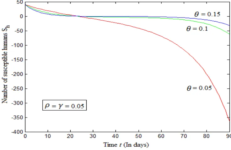
In the human susceptible population, as shown in Fig 2 to Fig 4, the solution of Sh using HPM for fixed values of
0.05, 0.1 and 0.15
γ ρ θ
= = =
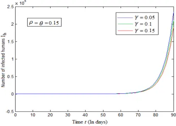
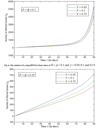
when the rate of vaccination value and Sh value also increased. If theeffectiveness of the use of anti-malarial drugs is increased, then it increases the number of susceptible humans as well as the number of recovered humans, but it decreases the number of infected humans. The use of anti-malarial drugs given to human has also an impact on the mosquito population, as shown in Fig 5 to Fig 7, the solution of Ih
using HPM for fixed values of
γ ρ θ
= = =
0.05, 0.1 and 0.15
when the rate of spraying increased and Ihdecreased in Human susceptible and Mosquito susceptible of anti-malarial drugs, vaccines and spraying.
The same treatment on causes a decrease in the number of infected mosquitoes but an increase in the number of susceptible mosquitoes. Increasing or decreasing in the number of humans and mosquitoes in each class tend to be equal to any increase in the effectiveness of the use of anti-malarial drugs. The maximum number of infected humans and mosquitoes occurs at =25 days. At this point, the effectiveness level of 20% can reduce the number of infected humans up to 23.81% of the total human population and can reduce the number of infected mosquitoes up to 5.88%. It is assumed that infected humans treated with anti-malarial drugs by 10%.
In this case, it will be shown the effect of parameters and the basic reproduction number 0 to the population
0.05, 0.1 and 0.15
γ ρ θ
= = =
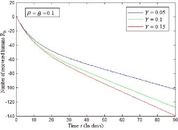
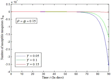
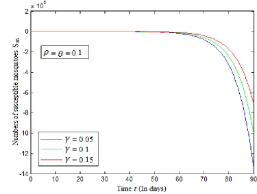
when the rate of spraying increased and Rh decreased in Human Infected,Mosquito Infected of anti-malarial drugs, if the effectiveness of the vaccine is improved and the other parameters are fixed, then the number of humans in susceptible and recovered classes is increased. It indirectly causes a decrease in the number of human in infected class. While, in the mosquito population as shown in Fig 11 to Fig 13, the solution of Sm using HPM for fixed values of
γ ρ θ
= = =
0.05, 0.1 and 0.15
when the rate of spraying value and Sm [image:5.595.124.492.175.415.2]value also increased in Human Infected, Mosquito Infected of vaccines, improvement on vaccine effectiveness indirectly decreases the number of mosquito in infected class.
Fig. 2: The solution of Sh using HPM for fixed values of
γ ρ
= =
0.05 and
θ
=
0.05, 0.1 and 0.15
[image:5.595.122.485.460.729.2]Fig. 4: The solution of Sh using HPM for fixed values of
γ ρ
= =
0.15 and
θ
=
0.05, 0.1 and 0.15
[image:6.595.123.485.395.654.2]Fig. 6: The solution of Ih using HPM for fixed values of
θ ρ
= =
0.1 and
γ
=
0.05, 0.1 and 0.15
Fig. 7: The solution of Ih using HPM for fixed values of
θ ρ
= =
0.05 and
γ
=
0.05, 0.1 and 0.15
Now we demonstrate the effectiveness of the use of spraying on human populations and mosquito populations. In this case we still assumed that infected humans consume anti-malarial drugs by 10% and we show the effect of parameter and 0 on population dynamics. In Fig. 5 Human Infected, Mosquito Infected of spraying, we can see that an
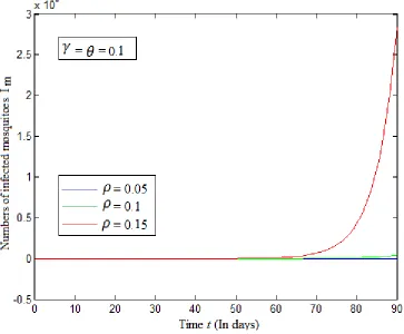
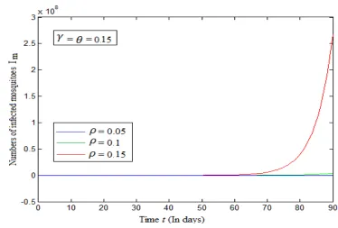
improvement on the effectiveness of spraying increases the number of susceptible humans, but decreases the numbers of infected mosquitoes and recovered humans. In Fig 14 to Fig 16, the solution of Im using HPM for fixed values of
0.05, 0.1 and 0.15
γ ρ θ
= = =
when the rate of spraying value and Im value also increased in Human RecoveredFig. 8: The solution of Rh using HPM for fixed values of
θ ρ
= =
0.15 and
γ
=
0.05, 0.1 and 0.15
[image:8.595.125.489.347.613.2]Fig.10: The solution of Rh using HPM for fixed values of
θ ρ
= =
0.05 and
γ
=
0.05, 0.1 and 0.15
[image:9.595.122.491.362.631.2]Fig. 12: The solution of Sm using HPM for fixed values of
θ ρ
= =
0.15 and
γ
=
0.05, 0.1 and 0.15
[image:10.595.122.488.393.616.2]Fig. 14: The solution of Im using HPM for fixed values of
θ γ
= =
0.05 and
ρ
=
0.05, 0.1 and 0.15
[image:11.595.129.492.361.661.2]Fig. 16: The solution of Im using HPM for fixed values of
θ γ
= =
0.15 and
ρ
=
0.05, 0.1 and 0.15
CONCLUSION
In this paper, we have presented an SIRS-SI model of malaria disease. The malaria model non-linear differential equations have been solved analytically and numerically. Simple and approximate dimensionless concentrations are derived by using the HPM for all values of dimensionless parameters. The HPM is an extremely simple method and it is also a promising method to solve other nonlinear equations. This method can be easily extended to find the solution of all other non-linear equations. This present method is quick and efficient and is able to significantly the amount of computations in simulations of this model.
APPENDIXA
Basic Concepts of the Homotopy Perturbation Method
The HPM method has overcome the limitations of traditional perturbation methods. It can take full advantage of the traditional perturbation techniques, so a considerable deal of research has been conducted to apply the homotopy technique to solve various strong non-linear equations. To explain this method, let us consider the following function:
r , 0 ) ( )
(u − f r = ∈Ω
Do (A1)
With the boundary conditions of
r , 0 ) u ,
( = ∈Γ
∂ ∂
n u
Bo (A2)
Where, D is a general differential operator, o B is a boundary operator, o f(r) is a known analytical function and Γ is the boundary of the domainΩ. Generally speaking, the operator D can be divided into a linear part o L and a nonlinear partN . Eq. (A1) can therefore be written as
0
)
(
)
(
)
(
u
+
N
u
−
f
r
=
L
(A3)By the homotopy technique, we construct a homotopy v(r,p):Ω×[0,1]→ℜ that satisfies
0 )] ( ) ( [ )] ( ) ( )[ 1 ( ) ,
(v p = −p L v −L u0 +p D v − f r =
0 )] ( ) ( [ ) ( ) ( ) ( ) ,
(v p =L v −Lu0 + pLu0 +p N v − f r =
H (A5)
Where p∈[0,1] is an embedding parameter , and u is an initial approximation of Eq. (A1) that satisfies the 0
boundary conditions. From Eqs. (A4) and (A5), we have
0 ) ( ) ( ) 0 ,
(v =L v −L u0 =
H (A6)
. 0 ) ( ) ( ) 1 ,
(v =D v − f r =
H o (A7) When p=0, Eq. (A4) and Eq. (A5) become linear equations. When p =1, they become non-linear equations. The process of changing p from zero to unity is that of L(v)−L(u0)=0 toDo(v)− f(r)=0. We first use the embedding parameter
p
as a “small parameter” and assume that the solutions of Eqs. (A4) and (A5) can be written as a power series inp
:...
2 2 10
+
+
+
=
v
pv
p
v
v
(A8)Setting p=1 results in the approximate solution of Eq. (A1):
.... v
lim 0 1 2
1 = + + +
=
→ v v v
u
p
(A9)
This is the basic idea of the HPM.
APPENDIXB
Solution of Nonlinear Differential Equations (1) - (5) Using HPM
In this appendix, we indicate how (6) – (10) in this paper are derived. To find the solution of (1) – (5), they can be simplified to
1 2 3
0
h
h h h h h m h
dS
R
a S I
b
S I
S
dt
− −
λ σ
+
β
+
β
+
θ
=
(B1)1 2 4
0
h
h h h h m h
dI
I
a S I
b
S I
I
dt
−
η
−
β
−
β
+
θ
=
(B2)2
0
h
h h h
dR
k I
R
S
dt
−
γ
+
θ
−
θ
=
(B3)3 1
0
m
m h m m
dS
c
I S
S
dt
−
λ
+
β
+
θ
=
(B4)3 1
0
m
h m m
dI
c
I S
I
dt
−
β
−
θ
=
(B5) where1 m
,
2 h,
3 h,
4 hk
θ µ
=
+
ρ θ
=
µ σ θ
+
=
µ θ θ
+
=
µ α γ
+ +
(B6)3 1 2 3
4 1 2 4
2 2
1
(1
)
0
(1
)
0
(1
)
0
(1
)
h h
h h h h h h h m h
h h
h h h h h h m h
h h
h h h h
m
m m
dS
dS
p
S
p
R
a S I
b
S I
S
dt
dt
dI
dI
p
I
I
p
I
a S I
b
S I
I
dt
dt
dR
dR
p
R
p
k I
R
S
dt
dt
dS
p
S
dt
λ θ
λ σ
β
β
θ
η
θ
η
β
β
θ
θ
γ
θ
θ
λ θ
−
− +
+
− −
+
+
+
=
−
−
+
+
−
−
−
+
=
−
+
+
−
+
−
=
−
−
+
3 11 3 1
0
(1
)
0
m
m h m m
m m
m h m m
dS
p
c
I S
S
dt
dI
dI
p
I
p
c
I S
I
dt
dt
λ
β
θ
θ
β
θ
+
−
+
+
=
−
−
+
−
−
=
(B7)The analytical solutions of the system (B1)-(B5) are 2
0 1 2
2
0 1 2
2
0 1 2
2
0 1 2
2
0 1 2
...
...
...
...
...
h h h h
h h h h
h h h h
m m m m
m m m m
S
S
pS
p S
I
I
pI
p I
R
R
pR
p R
S
S
pS
p S
I
I
pI
p I
=
+
+
+
=
+
+
+
=
+
+
+
=
+
+
+
=
+
+
+
(B8)Substituting (B8) into (B7) and comparing the coefficient of like powers of p in (B7), we get
0 0
3 0
0 0
0 4 0
0 0 2 0 0 0 1 0 0 0 1 0
:
0
:
0
:
0
:
0
:
0
h h h h h h h h m m m m mdS
p
S
dt
dI
p
I
I
dt
dR
p
R
dt
dS
p
S
dt
dI
p
I
dt
λ θ
η
θ
θ
λ θ
θ
− +
=
−
+
=
+
=
−
+
=
−
=
(B9) 1 10 1 0 1 2 0 0 3 1
1 1
1 1 0 0 2 0 0 4 1
1 1
0 2 1 0
1 1
3 0 0 1 1
1 1
3 0 0 1 1
:
0
:
0
:
0
:
0
:
0
hh h h h m h
h
h h h h m h
h
h h h
m
h m m
m
h m m
dS
p
R
a S R
b
S I
S
dt
dI
p
R
a S R
b
S I
R
dt
dR
p
k R
R
S
dt
dS
p
c
I S
S
dt
dI
p
c
I S
I
dt
σ
β
β
θ
η
β
β
θ
γ
θ
θ
(0)
40,
(0)
2,
(0)
0,
(0)
500,
(0) 10
( )
( )
( )
( )
( )
0,
1, 2,...,
h h h m m
h h h m m
S
I
R
S
I
S i
I i
R i
S i
I
i
i
=
=
=
=
=
=
=
=
=
=
=
∞
(B11)Solving (B9) and using the boundary conditions (B11), we obtain the following results.
3 0 3 3
40
t h h hS
λ
λ
e
θθ
θ
−
=
+
−
(B12)4
( )
0
2
t h
I
=
e
η θ− (B13)0
0
h
R
=
(B14)1 0 1 1
500
t m m mS
λ
λ
e
θθ
θ
−
=
+
−
(B15)1
0
10
t m
I
=
e
θ (B16)Solving (B10) and using the boundary conditions (B11), we obtain the following results.
3 ( 4 3) 1 ( 1 3)
1
4 1 3 1 4 1 3 1
1 2 2
3 3
where
40
,
10
,
10
40
t t t t
h
h h
A
B
C
A
B
C
S
e
e
e
e
A
a
B
b
C
b
θ η θ θ θ θ θ
η θ
θ θ
θ
η θ
θ θ
θ
λ
λ
β
β
β
θ
θ
− − − −
=
+
+
−
−
−
−
+
−
+
=
=
=
−
(B17) 4 3 1 1 1 3 1 ( )3 4 5 3
1 2
1 4 3 1 1 1 1 3 1 4 3
( ) 5
4
1 1 1 1 3
1 4 2 1 3 1 4 2 5
3 3 3
where
,
2
,
2
40
,
10
,
10
t D t D t
h
t t
h h h
D
D
D
D
I
e
tD e
e
D
D
D
D
D
D
e
e
D
D
D
D
a
D
a
D
b
D
η θ θ
θ θ θ
η θ θ
θ
θ θ
η θ θ
θ
θ θ
λ
λ
λ
θ η
β
β
β
θ
θ
θ
− − − − − −
= −
+
+
+
+
− − −
+
+ −
− − −
+
+
+
+ −
= −
=
=
−
=
=
2 340
hb
β
λ
θ
−
(B18) 3 2 43 ( ) 3
1
4 2 2 3 2 3 4 2 2 3 2 3
40
40
2
2
h h t t t h h hk
k
R
e
θe
η θe
θλ
λ
θ
θ
θ
θ
θλ
θλ
γ
γ
η θ θ θ θ
θ θ
−η θ θ
−θ θ
θ θ
−
−
−
= −
+
+
+
−
−
− +
−
− +
−
(B19)1 4 4 1
2 2
1 ( ) 1 ( )
2 2
1
1 4 1 4 1 1 4 1 4 1
2
500
2
500
2
2
(
)
2
(
)
2
m m
t t t
m m
m
c
c
c
c
S
e
θe
η θe
η θ θλ
λ
β
β
θ
θ
β λ
β λ
θ η θ θ
η θ
θ
θ η θ θ
−η θ
θ
− −
−
−
=
+
−
−
− −
− −
− −
− −
(B20)1 4 4 1
2 2 2
1 1 ( ) 1 ( )
2 1
1 4 1 4 1 4 1 4 1
2 5 0 0 2 2 5 0 0
2
( ) 2 2
m m m
t t t
m m
c c c
c
I eθ eη θ eη θ θ
λ λ λ
β β β
θ θ θ
β λ
θ η θ θ η θ θ η θ θ − η θ θ − −
− − = − − + + − − − − − − − − (B21)
0 1 2
0 1 2
0 1 2
0 1 2
0 1 2
lim 1 ( ) ...
lim 1 ( ) ...
lim 1 ( ) ...
lim 1 ( ) ...
lim 1 ( ) ...
h h h h h
h h h h h
h h h h h
m m m m m
m m m m m
S p S t S S S
I p I t I I I
R p R t R R R
S p S t S S S
I p I t I I I
= → = + + +
= → = + + +
= → = + + +
= → = + + +
= → = + + +
(B22)
Acknowledgments
The authors would like to thank the referees for their helpful comments, which improved the presentation of the paper.
REFERENCES
[1]FA Rihan; MN Anwar, International Journal of Differential Equations, 2012, 20 (1), 12-20. [2] H El Maroufy; L Omari; Z Taib, Stochastic Models, Taylor & Francis, 2012, 28 (1), 23-32. [3] JL Aron, Mathematical Biosciences, 1988, 90 (2), 385–396.
[4]CJ Struchiner; ME Halloran; A Spielman, Math Biosci., 1989a, 94 (1), 87–113. [5]ME Halloran; CJ Struchiner; A Spielman, Math Biosci., 1989b, 94 (2), 115–149. [6]IM Hasting; WM Watkins, Acta Tropica, 2005, 94 (4), 218–229.
[7]APP Wyse; L Bevilacquaa; M Rafikov, Ecological Modelling, 2007, 206 (3), 322–330.
[8]C Chiyaka; JM Tchuenche; W Garira; S Dube, Applied Mathematics and Computation, 2008, 195 (2), 641–662. [9]C Chiyaka; W Garira; S Dube, Theoretical Population Biology, 2009, 75 (4), 14–29.
[10]J Tumwiine; JYT Mugisha; LS Luboobi, Journal of Mathematical Analysis and Applications, 2010, 361 (1), 139– 149.
[11]L Wang; Z Teng; T Zhang, Commun Nonlinear Sci Numer Simulat., 2013, 18 (1), 1288– 1303. [12]GA Ngwa; WH Shu, Mathemaiical and Computer Modelling, 2000, 32 (2), 747–763.
[13]LS Pontryagin; VG Boltyanskii; RV Gamkrelidze; EF Mishchenko, Wiley New York, 1962. [14]Y Lou; XQ Zhao, Bull Math Biol., 2011, 73 (1), 384-407.
[15]TK Kar; A Batabyal, Biosystems, 2011, 104 (1), 127–135.
[16]JH He, Computer Methods in Applied Mechanics and Engineering, 1999, 178 (2), 257–262. [17]JH He, Applied Mathematics and Computation, 2003, 135 (1), 73–79.
[18]JH He, Applied Mathematics and Computation, 2003, 140 (2), 217–222. [19]PD Ariel, Nonlinear Science Letters, 2010, 1 (2), 43–52.
[20]QK Ghori; M Ahmed; AM Siddiqui, International Journal of Nonlinear Sciences and Numerical Simulation, 2007, 8 (2), 179–184.
[21]T Öziş; A Yildirim, International Journal of Nonlinear Sciences and Numerical Simulation, 2007, 8 (2), 243– 248.