Estimating parameters in the presence of many nuisance parameters

(1)

LONDON SCHOOL OF ECONOMICS

Estimating Parameters in the Presence

of Many Nuisance Parameters

by

Billy Wu

Thesis submitted in fulfilment for the

MPhil Degree

in the

Department of Statistics

Supervisor: Prof. Qiwei Yao

(2)

I, BILLY WU, declare that this report titled, ‘Estimating Parameters in the Presence

of Many Nuisance Parameters’ and the work presented in it are my own.

Signed:

Date:

(3)

Abstract

This paper considers estimation of parameters for high-dimensional time series with the

presence of many nuisance parameters. In particular we are interested in data consisting

ofptime series of lengthn, withpto be as large or even larger thann. Here we consider the composite-likelihood estimation and the profile quasi-likelihood estimation. The

asymptotic properties of these methodologies are investigated. Simulations are used to

illustrate our both of these methods and explore the performance of these methods.

Key words: composite likelihood, nuisance parameter, profile likelihood, quasi-likelihood,

(4)

I would like to thank my advisor Professor Qiwei Yao, he gave me a huge amount of

support and guidance. He has a seemingly endless well of knowledge and an incredible

amount of patience. I hope to one day repay his immeasurable amount of help.

I would also like to thank my family for their all their support. I owe them a great deal

for everything in my life, and for making me the person I am today. My parents and

my grandparents raised me and nurtured me, I have had an incredible life experience.

They always had my best interests at heart and worked extremely hard to give me the

best opportunities available, I will forever be grateful.

Last but not least I would also like to thank all my friends. Without their moral

support and friendship, my entire life would not be the same. I am fortunate to have

such amazing friends.

(5)

Introduction

1.1 Introduction

Rapid developments in technology in this information age has led to data collection in an

unprecedentedly large scale. This brings a new opportunity with challenge to statistics.

The availability of large data sets enable statisticians to look into complex structures

using sophisticated models. In this paper we consider a class of models in which the

number of parameters of interest is finite while the number of nuisance parameters is

large or excessively large in relation to the sample size. Those models arise in various

statistical applications. For example, in a longitudinal model with a large number of

sites the primary interest lies in a small number of parameters representing the common

effects while the individual levels of different sites are treated as nuisance parameters. For

a large panel of time series data, one is often interested in a few common factors which

drives the dynamics of all the component series and treats the parameters representing

each idiosyncratic components as nuisance parameters. In the attempts to model the

volatilities of large number of financial securities, it is often to assume that the dynamic

volatilities are controlled by a small number of parameters in the presence of large

number of nuisance parameters representing marginal covariance matrices.

In this paper we consider two methods to obtain the estimators of a fixed number of

pa-rameters of interest in presence of a large number of nuisance papa-rameters. The methods

concerned are the maximum profile quasi-likelihood estimation (MPQLE) and the

maxi-mum composite quasi-likelihood estimation (MCQLE). With an initial estimator for the

nuisance parameter vector, the MPQLE maximises a profile quasi-likelihood function to

obtain the estimation. This is in line with more conventional approach. By plugging in

an initial estimator for the nuisance parameters, we avoid a maximisation problem with

(7)

Chapter 1. Introduction 2

a large number of variables. However it is intuitively clear that the quality of the initial

estimator impacts on the ultimate outcome of the procedure.

Another method to be considered is the composite likelihood, the name coined by

Lind-say (1988). See also a recent survey Varin et al. (2011). A composite likelihood is

a function derived by multiplying a collection of, typically two- or there-dimensional,

marginal density functions. In our context, each low dimensional density function only

depends on a small number of nuisance parameters, hence can be easily profiled. The

resulting composite profile likelihood function depends on those parameters of interest

only, can be solved to obtain the estimator without running into high-dimensional

opti-misation problems. Because the marginal densities are multiplied together, ignoring the

original distribution structure, the MCQLE can be viewed as derived from a (seriously)

misspecified model.

The major contribution of this paper is the establishment of the asymptotic properties for

both the MCQLE and the MPQLE under the condition which is relevant to the settings

concerned. The conventional asymptotic theory is typically under the assumption that

the sample size goes to infinity while everything else remains fixed. For our setting,

the number of nuisance parameters is of a comparable magnitude of the sample size.

Hence it is more pertinent to consider the asymptotics when both the sample size and

the number of nuisance parameters go to infinity together. Though bearing a similar

banner, our theory is different from large literature on the theory for the so-called ‘large

pand small n’ regression problem; see, among the others, Zou (2006), Fan and Lv (2008), Huang et al (2008), Zhang and Huang (2008), Bickel et al (2009) and Zhang (2009).

The name of ‘composite likelihood’ was introduced by Lindsay (1988), although the

idea of using ‘submodels’ or ‘marginal models’ had appeared before. As the full

lihood with complex models are often computationally infeasible, The composite

like-lihood methods have been used in different regression with dependent errors (Eicher

1967), problems including modelling spatial processes (Besag 1974), case control studies

(Liang 1987), inference for nonlinear dynamic models (Gallant and White 1988),

cor-related binary data (Kuk and Nott 2000), grouped data (deLeon 2005), longitudinal

studies (Molenberghs and Verbeke 2005), multivariate volatility modeling (Engle et al.

2008), bioinformatice (Larribe and Fearnhead 2011). The asymptotic theory under the

assumption that only sample size tends to infinity has been studies by, for example,

Cox (1961), Eicher (1967), White (1982), Gallant and White (1988), and Cox and Reid

(2004). To our knowledge, no results have been derived under our setting when both the

sample size and the number of nuisance parameters go to infinity together. For more

comprehensive survey in the composite likelihood methodology, we refer to the first issue

(8)

The rest of the paper is organised as follows. Section 2 deals with the MCQLE and

section 3 is on MPQLE. In each of those two sections, we outline the method and

state the asymptotic normality results. Both the methods are illustrated in simulation

(9)

Chapter 2

Methodology

2.1 Composite-likelihood estimation

Let {X1,· · · ,Xn} bep×1 observations from a stationary process with the underlying

distribution depending on parameter (θ,ω)∈Θ×Ω⊂Rd+q_{, where}_θ_{is a}_d_×_{1 parameter}

of interest, andωis aq×1 nuisance parameter. Our goal is to estimateθ. We consider now a maximum composite quasi-likelihood estimation method forθ. We will show that

such an estimator is asymptotically normal with the standard root-n convergence rate

asn, q → ∞together while dis fixed, andp may also diverge to infinity.

Let Xt1,· · ·,Xtr be r subvectors of Xt. The lengths of those r subvectors may be

different from each other, and some of those subvectors may share common components

from Xt. With the observations Xtj, t = 1,· · ·, n, the log marginal quasi-likelihood

function is defined as

lj(θ,ωj) = n

X

t=1

logfj(Xtj;θ,ωj),

which depends on the parameter of interest θ, and a subset of nuisance parameter

denoted by ωj. Let

e

ωj(θ) = arg max

ωj

lj(θ,ωj). (2.1.1)

We define a composite quasi-likelihood function forθ as

l(θ) =

r

X

j=1

lj θ,ωej(θ)

. (2.1.2)

The maximum composite quasi-likelihood estimator (MCQLE) for θ is defined as

b

θ= arg max

θ l(θ). (2.1.3)

(10)

We assume that r=r(q)→ ∞ asq→ ∞, while all the lengths of Xtj and ωj are fixed.

One implicit condition for the MCQLE defined in (2.1.3) being reasonable is that the nuisance parametersω1,· · · ,ωrare distinct from each other such that the maximisation

(2.1.1) may be carried out independently for eachjwithout confounding constraints from each other. This is a rather strong requirement, and may only be facilitated by selecting

subvectors Xt1,· · · ,Xtr in a restrictive manner. It is very likely there may be a heavy

loss of information if we adhere to this requirement in practice. One alternative is to

adopt the so-called ‘variation-free’ condition imposed by Engle, Hendry and Richard

(1983), which ignores the links among different ωj and treats ω1,· · · ,ωr as different

and unconnected nuisance parameters. See also Engle, Shephard and Sheppard (2008).

Of course there will be some efficiency loss in estimation of θ resulted from neglecting

the links among different ωj. The trade-off is that we will be able to reduce an extra

high-dimensional optimisation problem to many low-dimensional problems, which is the

essential motivation of using composite-likelihood approach. Note that this

variation-free condition also implies thatbθ is the global maximiser in the sense that

(bθ, b

ω1, · · · , ωbr) = arg max

θ,ω1,···,ωr

r

X

j=1

lj(θ,ωj),

where we treat ω1,· · ·,ωr as different and independent parameters. In the rest of this

section, we always adopt this assumption.

Letβ= (θ0,ω0₁,· · ·,ω0_r)0, andl(β) =Pr

j=1lj(θ,ωj).In practice we takeβb = (θb

0 ,ωb

0

1,· · · ,ωb

0

r)0

as a solution of the likelihood equation

˙ l(βb) ≡

∂ ∂βl(β)

_β₌

b

β = 0. (2.1.4)

Let

β_o≡(θ0_o,ω0₁_o,· · · ,ω0_ro)0 = arg max

θ,ω1,···,ωr E{

r

X

j=1

logfj(Xtj;θ,ωj)} (2.1.5)

be the true value of the parameter, which is assumed to be an inner point of the

param-eter space. Put

atj(θ,ωj) =

∂

∂θlogfj(Xtj;θ,ωj), btj(θ,ωj) = ∂ ∂ωj

logfj(Xtj;θ,ωj),

Atj(θ,ωj) =

∂2

∂θ∂θ0 logfj(Xtj;θ,ωj), Btj(θ,ωj) = ∂2

∂θ∂ω0_j logfj(Xtj;θ,ωj),

Ctj(θ,ωj) =

∂2 ∂ωj∂ω0_j

(11)

Chapter 2. Methodology 6

We simply writeatj=atj(βo,ωjo), andbtj,Atj,Btj and Ctj in the same manner. Put

M1 =−

       Pr

j=1EAtj EBt1 · · · EBtr EB0_t₁ ECt1

..

. . ..

EB0_tr ECtr

       , (2.1.6)

M2=−

       1 r Pr

j=1EAtj 1 √

rEBt1 · · ·

1 √

rEBtr

1 √

rEB

0

t1 ECt1 .. . . .. 1 √ rEB 0

tr ECtr

       , (2.1.7)

and the elements at the blank places in the above matrices are 0.

We introduce some regularity conditions first.

A1 {Xt}satisfies the mixing condition stated in C3 in the Appendix.

A2 fj are smooth enough such that all the required derivatives exist and are continuous

and integrable whenever necessary.

A3 Denote byξtj any component ofatj, andηtj any component ofbtj. Forν >2 given

in A1 above, it holds that

lim

r→∞E

1 r r X j=1 ξtj ν

<∞, (2.1.8)

lim r→∞ 1 r r X j=1

[E(η_tj2) +{E(|ηtj|ν)}2/ν]<∞. (2.1.9)

By Hlder’s inequality this is equivalent to

lim r→∞ 1 r r X j=1

[E(|ηtj|ν)2/ν]<∞. (2.1.10)

A4 Denote byηtj any element of Atj−E(Atj), Btj−E(Btj) orCtj−E(Ctj). Then

(2.1.9) holds.

A5 The matrix M1 is positive-definite. Furthermore all the eigenvalues of the matrix

M2 are bounded above from ∞and below from 0, asr → ∞.

A6 There exists a constantc1>0 and positive functionsλj(·) such that| ∂

3

∂β`∂βi∂βklogfj(xj;θ,ωj)| ≤ λj(xj) for any||θ−θo|| ≤c1and||ωj−ωjo|| ≤c1. Furthermore limr→∞sup₁≤j≤rE{λj(Xtj)}<

(12)

A7 (2.1.9) holds with ηtj being any component of ζtj ≡ atj −E(B1j)(EC1j)−1btj.

Furthermore the limits of the convariance

Wk = limr→∞_r12

Pr

j=1ζ1j,

Pr

j=1ζk+1,j

, k= 0,1,· · · , n.Exists

Remark 1. (i) Note that M1 = −E

n

∂2

∂β∂β0

Pr

j=1logfj(Xtj;θ,ωj)

o

. The condition

that M1 > 0 in A5 implies that βo, defined in (2.1.5), is an isolated maximiser. It

also implies that M2 is positive-definite as M2 = ΛM1Λ, where Λ is an appropriate

full-ranked diagonal matrix.

(ii) If X1,· · ·,Xn are independent observations, conditions A3, A4 and A6 may be

reduced to those withν = 2 only.

2.1.1 Theorem 1

Theorem 1. Let conditions A1 – A6 hold. Then there exists a solution of the likelihood

equation (2.1.4) for which

m||bθ−θ_o||2+

1 r

r

X

j=1

||ω_bj −ωjo||2 P

−→0

for any m→ ∞,r/m→0 andr2m/n→0.

Remark 2. The convergence rates in Theorem 1 are not optimal; see, for example,

The-orem 2 below which indicates that the convergence rate for bθ is root-n. The important

message here is the difference in the convergence rates betweenbθand{ b

ωj, j= 1,· · · , r}.

Asr → ∞together withn, the rate for the uniform convergence ofω1b ,· · · ,ωbr is slower.

It also imposes some restrictions on the number of parameters which can be consistently

estimated, although the implied rates such asr =o(n1/3) is presumably too restrictive. In region of the true parameter if there is a unique solution then this would be the true

min.

2.1.2 Theorem 2

Theorem 2. Let conditions A1 – A7 hold, matricesE(C1j),j= 1,· · ·, r, be invertible,

and the limit of M2, defined in (2.1.7), exist (as r → ∞). Furthermore, let r/n → 0. For any consistent solution of the likelihood equation (2.1.4) in the sense that

||θb−θ_o||2+

r

X

j=1

||ω_bj−ωjo||2 P

(13)

it holds that

√

n(θb−θ)

D

−→N

0, L−1 W0+ 2 ∞

X

k=1 Wk

L−1

,

whereWkare defined in A7, andL= limr→∞r−1Pr_j₌₁{E(A1j)−E(B1j)(EC1j)−1E(B0₁_j)}.

Remark 3. (i) The consistence condition (2.1.10) is weaker than that identified in Theorem 1, asm/r→ ∞.

(ii) The limit which defines the matrix L exists. This is implied by the existence of the

limit of M2.

2.2 Profile quasi-likelihood estimation

We consider now the asymptotic properties of a qMLE for θ, obtained based on a

reasonable initial estimator for the nuisance parameterω. We will show that the qMLE

is asymptotically normal with the standard root-n convergence rate in spite that the

number of nuisance parameters q goes to∞.

We use a log quasi-likelihood function

l(θ, ω) =

n

X

t=1

logf(Xt;θ,ω), (2.2.12)

wheref is a density function defined onRp. With an initial estimatorω_b for the nuisance parameterω, a profile quasi-likelihood function forθ is defined as

l(θ) =

n

X

t=1

logf(Xt;θ,ωb),

and the maximum profile quasi-likelihood estimator (MPQLE) is defined as

e

θ= arg max

θ l(θ) = arg maxθ

n

X

t=1

logf(Xt;θ,ωb).

Let (θo,ωo) = arg maxθ,ωE{logf(Xt;θ,ω)}be the true parameter values. Since ˙l(eθ) =

0, it follows a Taylor expansion that

√

n(eθ−θ_o) = −

1

nm

¨_l(_θ?₎ −1 1 m√n

˙

l(θo), (2.2.13)

(14)

We introduce the regularity conditions first. Let

˙

l(θ) = ∂l(θ) ∂θ ,

¨

l(θ) = ∂ 2_l(_θ₎

∂θ∂θ0, a(x;θ,ω) = ∂

∂θlogf(x;θ,ω),

B(x;θ,ω) = ∂ 2

∂θ∂θ0logf(x;θ,ω), C(x;θ,ω) = ∂2

∂θ∂ω0 logf(x;θ,ω), and D(θ,ω) =E{C(Xt;θ,ω)}.

B1 The initial estimator ωb = (ωb1,· · · ,ωbq)

0 _{is asymptotically linear in the sense that}

for each 1≤j≤q,ω_bj−ωjo= _n1

Pn

t=1gj(Xt) +oP(n−1/2), where E{gj(Xt)}= 0,

Var{gj(Xt)} ≤ c < ∞, and c > 0 is a constant independent of j. Furthermore

||ω_b−ωo||2=OP(q/n), andq/n→0.

B2 f(x;θ,ω) is smooth such that all the required partial derivatives exists and are continuous. Denoted by aj the j-th component of a. There exists a positive

number c1 and a positive functionλ1(·)

such that

u

0∂2aj(x;θo,ω)

∂ω∂ω0 u

≤λ1(x)||u||

2 _{for any} _||_ω₋_ω

o|| ≤c1, u∈Rq and 1≤j≤q,

and E{λ1(Xt)} is bounded (asq → ∞). Furthermoreq/(m

√

n)→0.

B3 {Xt}satisfies condition C1 in the Appendix, and

ψn(Xt,Xs) ={C(Xt;θo,ωo)g(Xs) +C(Xs;θo,ωo)g(Xt)}/m

satisfies condition C2.

B4 For someγ >2 andγ > δ0given in C1, limq→∞E{||a(Xt;θo,ωo)+2D(θo,ωo)g(Xt)||γ}/mγ <

∞.Furthermore

Σj ≡ lim q→∞

1

m2Cov{a(X1;θo,ωo)+2D(θo,ωo)g(X1), a(X1+j;θo,ωo)+2D(θo,ωo)g(X1+j)}

exists for allj≥0.

B5 Letbij(x;θ,ω) be the (i, j)-th element ofB(x;θ,ω). There exist a positive number

c2 and a positive function λ2(·) such that ||_∂∂_θbij(x;θ,ω)||+||_∂∂_ωbij(x;θ,ω)|| ≤

λ2(x) for any ||θ −θo|| ≤ c2, ||ω −ωo|| ≤ c2 and 1 ≤ i, j ≤ d, the limit of

E{bij(Xt;θo,ωo)}/mexists, and bothE{λ2(Xt;θo,ωo)ν}/mν andE{bij(Xt;θo,ωo)ν}/mν

are bounded (as q→ ∞), where ν >2 is given as in C3. Furthermore,eθ

P

(15)

2.2.1 Theorem 3

Theorem 3. Under conditions B1-B5,√n(eθ−θ_o) is asymptotically normal with mean 0

and covariance matrixM−1(Σ0+2P∞j=1Σj)M−1, whereM= limq→∞E{B(Xt;θo,ωo)}/m >

(16)

Numerical Properties

3.1 Example 1

One-way error component model for panel data(Baltagi 2005, Chapter 2). Let

Ytj =µ+X0tjβ+µj+εtj, t= 1,· · ·, n; j = 1,· · · , r.

In the above modelYtj is the observation on thej-th individual at the timet,Xtj is the

k×1 observation onkexplanatory variables,µj denotes the individual-specific effect,εtj

are i.i.d. noise with mean 0 and variance σ2_{. To make the parameters identifiable, we} assume that P

jµj = 0. Suppose that we are interested in the effect of the explanatory

variables on individuals. Therefore we would like to estimateβandµ, treatingµ1,· · · , µr

as nuisance parameters. We consider the case that r is large in relation to nwhile k is fixed.

The conventional approach is to treatµj i.i.d. from an unknown distribution. Then the

MCQLE may be viewed as a conditional inference on µj. It is interesting to compare

the two approaches.

As an example, Ytj could be a country’s GDP. Xtj are explanatory variables for each

country j at year t such as population, literacy rate, unemployment rate etc. We are interested in the parameters µ and β for the linear regression Ytj = µ+X0tjβ. The

time-invariantµj accounts for any idiosyncratic domestic productivity. An example of

µj could be the amount the j-th country’s GDP is boosted by the timber which its

sub-tropical climate produces, assuming sustainable cutting and re-planting of trees this

constant boost is time-invariant and specific to this country. We are not interested in

such country specific factors and treat it as a nuisance parameter.

(17)

We will conduct a Monte Carlo simulation with 1000 repetitions. Newton Raphson

algorithm will be used to solve the likelihood equations for this and all subsequent

examples. First we generate β as random numbers from U(−1,1). Next we generate

µj ∼ N(0,1), we then constructµ= 1_r

Pr

j=1(µj). We transformµj →µj−µso that the

condition P

jµj = 0 is satisfied. We then generate Xtj where each element is a random

number fromN(0,1), let ¯Xj = _n1Pn_t₌₁(Xtj). We will transformXtj →Xtj−X¯j so that

the new Xtj satisfy the condition _n1 Pnt=1(Xtj) = 0. Finally we generate the dependent

variableYtj =µ+X0tjβ+µj +εtj by adding the i.i.d noiseεtj ∼ N(0,1).

We wish to minimise the log likelihood function of the form

l(µ,β,µ) =_b −1

2

X

j

X

t

(Ytj−µ−Xtj0 β−µj)2,

FOR MCQLE we will use 2 different approaches. First we pick all subsets (Xti,Xtj) for

1≤i6=j ≤r. The number of subsets isr(r−1)/2 and will grow rapidly as r increases, which is computationally costly. Our second approach we will pick consecutive subsets

of (Xti,Xtj) with 1≤i≤r−1, andj =i+ 1.

For MPQLE we’ll need to find an initial estimator bµj.

1 n

n

X

t=1

(Ytj) =µ+

1 n

n

X

t=1

(X_tj0 β) +µj +

1 n

n

X

t=1 (εtj),

Since we constructedXtj such that _n1 Pnt=1(Xtj) = 0 andεtj ∼ N(0,1) we have:

1 n

n

X

t=1

(Ytj) =µ+µj,

µ= 1 n

1 r

n

X

t=1

r

X

j=1 (Ytj),

b

µj =

1 n

n

X

t=1

(Ytj)−

1 n

1 r

n

X

t=1

r

X

(18)

[image:18.596.111.543.123.409.2]

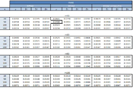
Table 1: The root mean square error of the methods over 1000 replications. n is the

number of observation, and r the number of nuisance parameters.

The results above illustrate the nice ”blessings of dimensionality”. As r increases the number of nuisance parameteresµj also increases, however the additional ”information”

available improves our estimates forµand β. Asn the number of observations increase we see improvements in our estimators as we would expect. The main hinderance to the

accuracy of our estimator would come from an increase ink, the number of explanatory variables.

The performance of MPQLE and MCQLE is very similar at all nandr, it is important to remember that the performance of MPQLE depends heavily on the quality of the

initial estimator, for this example our initial estimator is very good.

The quality of estimators from MCQLE and MCQLE consecutive are very close across all

(19)

3.2 Example 2

Scalar BEKK model(Engle, Shephard and Sheppard 2008). Let us considerp×1 return series Xt defined by

Xt=H1t/2εt, εt∼i.i.d.(0, Ip), (3.2.1)

Ht= (1−α−β)Σ+αXt−1X0t−1+βHt−1, (3.2.2)

whereα, β > 0 are dynamic parameters, α+β <1,Σ≡(σij)>0 is the unconditional

covariance matrix of Xt. Note that the model admits a strictly stationary solution.

Our interest is to estimate the dynamic parameters α and β while σij play the role of

nuisance parameters. It may be shown that (3.2.2) admits the solution

Ht=

1−α−β 1−β Σ+α

∞

X

j=1

βj−1Xt−jX0t−j. (3.2.3)

Assumingεt∼N(0,Ip), the log-likelihood function is of the form

l(α, β,Σ) =−1

2

X

t

(log|Ht|+X0tH

−1

t Xt),

which involves both the inverse and the determinant ofp×pmatrices Ht.

For MCQLE, we may consider two options: using all binary pairs (Xti, Xtj) for all

1≤i6=j≤p, or using only the consecutive pairs (Xti, Xt,i+1) for i= 1,· · ·, p−1. For MPQLE, we use the initial estimator

b

Σ= 1 n

n

X

t=1

(Xt−X)(X¯ t−X)¯ 0,

where ¯X=n−1P

tXt.

First we generate a random unconditional covariance matrixσ, steps are made to ensure it is positive semi-definite. We explicitly choose true values of α and β in the region of the empirical values of α and β when using the BEKK model on equity indices such as DAX30, FTSE100, S&P500, in a similar fashion to Engle, Shephard and Sheppard

2008.

(α, β) = (0.1,0.8),(0.05,0.93),(0.02,0.97) andp= 5,10,50,100, n= 2000.

Then we will generateXtandHtstepwise. During our estimation we use the constraint

(20)

For MCQLE, we may consider two options: using all binary pairs (Xti, Xtj) for all

1≤ i6=j ≤p; we call this MCQLEA, or using only the consecutive pairs (Xti, Xt,i+1) fori= 1,· · · , p−1 we call this MCQLEB. For MPQLE, we use the MLE of the covariance matrix as the initial estimator for Σ. Since we use the sample covariance matrix as anb

initial estimator the conditions for theorem 2 is met.

b

Σ= 1 n

n

X

t=1

(Xt−X)(X¯ t−X)¯ 0,

where ¯X=n−1P

(21)

[image:21.596.175.459.157.448.2]

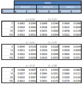
Table 2: Root mean square error of the methods over 500 replications. Where the

number of observationn is fixed at 1000, and different values are taken for the number of nuisance parametersp. 3 Sub-tables with different true values for the parameters we wish to estimate.

From the table above we can see for both MCQLEA and MCQLEB we gain performance

with the increase of dimensionality inp, however for MPQLE whenpincreases and gets closer to the size of n the quality of estimators starts to get worse. We will further investigate the impact on all 3 approaches when the size of p is large compared to n with another simulation shown below.

MCQLEB does not perform as well as MCQLEA when the dimension pof Xt is small,

but in the cases where p is large there are no significant differences in performance. However the number of subset pairings of MCQLEA is p(p−1)/2 while MCQLEB only havep−1 pairs. The huge increase of computational cost of MCQLEA is not justified for reasonably largep. In some situations, for example indices derivatives trading, a decision or price quotation could be extremely time sensitive, it may be worth investigating

what impact reducing the number of pairings even further could have. We saw similar

results in example 1 in terms of the computational cost benefits of not choosing subsets

(22)

[image:22.596.173.459.123.413.2]

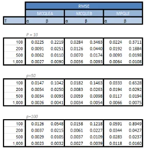
Table 3: We perform 500 replications where each sub-table has a fixed number of

nui-sance parametersp, with the number of observationsT ranging from 100 to 1000.

We perform further simulations to cross examine how the estimation methods compare

with each other when p is large in relation to n. We will perform 500 replications for each simulation. We use the values α = 0.03 and β = 0.95, p = 10,50,100 and t= 100,200,500,1000

The results above show that the increase innimproves our estimators for all 3 approaches as we would expect, since more information from an increase of observations would yield

(23)

Chapter 4

Proofs

We use the same notation as in chapter 2.

4.1 Proof of Theorem 1

The basic idea in the proof of Theorem 1 is the same as that of Theorem 6.5.1 of

Lehmann and Casella (1998), although it becomes technically much more involved in

order to handle the increasing number of parameters asn→ ∞.

Let

Qδ=

(θ,ω1,· · · ,ωr)

||θ−θ_o||2+

1 r

r

X

j=1

||ωj−ωjo||2=δ2/m .

We will show that for any δ > 0 fixed, l(β) < l(β_o), for all β ∈ Qδ, with probability

converging to 1. Therefore with probability arbitrarily close to 1 l(β) attains a local maximum in the interior ofQm for all sufficiently large n. Letβb be the local maximum

closest to β₀. By the above argument, βb must lie in the interior of Q_δ for any δ > 0.

This entails the required assertion.

To establish the needed fact concerning the behaviour of l(β) on Qδ, we evoke a Taylor

expansion:

1

nr{l(β)−l(βo)} = 1

nr(β−βo) 0_˙

l(β_o) + 1

2nr(β−βo) 0_¨

l(β_o)(β−β_o)

+ 1

6nr

X

`,i,k

(β`−β`o)(βi−βio)(βk−βko)

∂3 ∂β`∂βi∂βk

l(β?) ≡ S1+S2+S3(4.1.1),

whereβ? lies between βand β_o.

(24)

For β∈Qδ, write θ−θo= √δ_mγ and ωj −ωjo=δp_mrγj. Then all the elements of γ

and γ_j are between−1 and 1. Furthermore,

S1 = δγ0 n√m

n X t=1 1 r r X j=1 atj+

δ√r n√m

n X t=1 1 r r X j=1

γ0_jbtj. (4.1.2)

Letξtj denote any component of atj. Since E(Pjatj) = 0, it holds for any >0 that

P √ m n n X t=1 1 r r X j=1 ξtj > ≤ m n2

Var(ζtr) + 2 n−1

X

t=1 (1− t

n)Cov(ζ1r, ζ1+t,r)

≤ m

n2

Var(ζtr) + 2E(|ζtr|ν)2/ν

∞

X

t=1

α(t)1−2/ν →(4.1.3)0.

whereζtr =r−1P1≤j≤rξtj. The last inequality follows from Proposition 2.5 of Fan and

Yao (2003); see also conditions A1 and A3. Hence the first sum on the RHS of (4.1.2) is of the orderoP(m−1), and the convergence is uniform for γ in any compact subset of

Rd_.

To estimate the second term on the RHS of (4.1.2), let dj denotes the length of btj ≡

(btj1,· · · , btjdj)

0_{. Then max}

1≤j≤rdj are bounded (as r→ ∞). Note

sup {γj}

n X t=1 r X j=1 γ0_jbtj

= sup

{γj}

r

X

j=1 γ0_j

n X t=1 btj ≤ r X j=1 dj X i=1 n X t=1 btji . Hence P sup {γj}

√ rm n n X t=1 1 r r X j=1 γ0_jbtj

> ≤ P √ rm n r X j=1 dj X i=1 n X t=1 btji > r ≤ r X j=1 P √ rm n dj X i=1 n X t=1 btji

> } ≤

r X j=1 dj X i=1 P √ rm n n X t=1 btji

> /d_j}

≤ rm(maxjdj)

2 n2 r X j=1 dj X i=1

{Var(btji) + 2(E|btji|ν)2/ν

∞

X

t=1

α(t)1−2/ν} →0, (4.1.4)

as r2m/n → 0 and condition A3 stands. The last inequality in the above expression follows the same argument as for (4.1.3). This shows that the second sum on the RHS of (4.1.2) is alsooP(m−1). ThereforeS1 =oP(m−1), and the convergence is uniform for

(25)

Chapter 4. Proofs 20

To calculateS2, we first note that similar to (4.1.4), condition A4 implies that 1 nr n X t=1 r X j=1

(θ−θo)0Atj(θ−θo)−

1 r

r

X

j=1

(θ−θo)0E(A1j)(θ−θo)

= 1 n n X t=1 1 r r X j=1

(θ−θo)0(Atj−EAtj)(θ−θo) =oP(m−1),

1 nr n X t=1 r X j=1

(θ−θo)0Btj(ωj−ωtj)−

1 r

r

X

j=1

(θ−θo)0E(B1j)(ωj−ωtj) =oP(m−1),

1 nr n X t=1 r X j=1

(ωj−ωtj)0Ctj(ωj−ωtj)−

1 r

r

X

j=1

(ωj −ωtj)0E(C1j)(ωj−ωtj) =oP(m−1).

Furthermore, all the convergences above are uniform for β ∈ Qδ, as the sizes of all

the matrices on the LHS of in the above expressions are fixed, and the the uniform

convergence may be established in the same manner as in (4.1.4). Now

S2 = 1 2nr n X t=1 r X j=1

{(θ−θo)0Atj(θ−θo) + 2(θ−θo)0Btj(ωj−ωjo) + (ωj−ωjo)0Ctj(ωj−ωjo)}

= 1 +oP(1) 2r

r

X

j=1

{(θ−θo)0EAtj(θ−θo) + 2(θ−θo)0EBtj(ωj−ωjo) + (ωj−ωjo)0ECtj(ωj−ωjo)}

=− 1

2r(β−βo) 0

M1(β−βo){1 +oP(1)}=−

1 2β

0

rM2βr{1 +oP(1)},

whereM1,M2 are defined in (2.1.6) and (2.1.7), and

β_r = ((θ−θo)0,(ω1−ω1o)0/

√

r,· · ·,(ωr−ωro)0/

√

r)0.

Forβ∈Qδ,||βr||2 =δ2/m. Since all the eigenvalues of M2 are bounded between 0 and

∞ (see condition A5),β0_rM2βr = 2c||βr||2 = 2cδ2/m, wherec >0 is a constant. Hence

(26)

Finally we deal with S3. Note that ∂

2

∂ωi∂ω0jl(β) = 0 for anyi

6

=j. Similar to the above, it may be proved using condition A6 that

|S3| ≤

1 +oP(1)

6r

X

`,i,k

(θ`−θ`o)(θi−θio)(θk−θko)

r

X

j=1

E{λj(Xtj)}

+ X

i,k

(θi−θio)(θk−θko)

r X j=1 X `

(ωj`−ωj`o)

E{λ_j(X_tj)}

+ X

k

(θk−θko)

r X j=1 X `,i

(ωj`−ωj`o)(ωji−ωjio)

E{λj(Xtj)}

+ r X j=1 X `,i,k

(ωj`−ωj`o)(ωji−ωjio)(ωjk−ωjko)

E{λ_j(X_tj)}

≡ (S31+S32+S33+S34){1 +oP(1)}.

Note that E{λj(Xtj)} is bounded by a constant for 1 ≤j ≤r, |θi−θio| ≤δ/

√

m and

|ωjk−ωjko| ≤δ

p

r/mfor allβ∈Qδ, and all the lengths ofωj are bounded. It is easy to

seeS31=O(m−3/2) =o(m−1) and S32=O(m−3/2r1/2) =o(m−1). On the other hand,

S33 ≤ c2 r√m

r X j=1 X `,i

(ωj`−ωj`o)(ωji−ωjio)

=

c2 r√m

r X j=1 X i

(ωji−ωjio)

2

≤ c3

r√m

r

X

j=1

||ωj−ωjo||2 ≤

c3

m3/2 = o(m −1_),

S34≤ c4 √ mr r X j=1 X i

(ωji−ωjio)

2

≤ c5r

1/2

m3/2 =o(m −1_).

This concludes that S3=oP(m−1).

Combining the above asymptotic approximations for S1, S2 and S3 together, we have shown that uniformly for β∈Qδ

1

nr{l(β)−l(βo)}=−c δ

2_/m₊_o

P(m−1),

wherec >0 is a constant. This completes the proof.

4.2 Proof of Theorem 2

Since ˙l(βb) = 0, it follows from a simple Taylor expansion that

b

(27)

where ¨l= _∂_β∂_∂2l_β0, and β? lies on the line betweenβb and β_o. Note

¨ l(β) =

n X t=1        Pr

j=1Atj(θ,ωj) Btj(θ,ω1) · · · Btr(θ,ωr) Bt1(θ,ω1)0 Ct1(θ,ω1)

..

. . ..

Btr(θ,ωr)0 Ctr(θ,ωr)

       ,

where the entries at the blank places are all 0. We partition the above matrix into

2×2 blocks withP

t

P

jAtj(θ,ωj) as the (1,1)-th block. By inverting this partitioned

matrix, the first dcomponents of (4.2.5) may now be expressed as

√

n(θb−θ_o)

= −n 1

nr r X j=1 _Xn t=1

Atj(θ?,ω?j)− n

X

t=1

Btj(θ?,ω?j)

n

X

t=1

Ctj(θ?,ω?j)

−1Xn

t=1

Btj(θ?,ω?j)

0o−1

× √1

n r r X j=1 Xn t=1 atj−

n

X

t=1

Btj(θ?,ω?j)

n

X

t=1

Ctj(θ?,ω?j)

−1Xn

t=1 btj

. (4.2.6)

For any matrix B, denote by |B|_a the sum of the absolute values of all the elements of B. Note that all the sizes of the matricesAtj, Btj andCtj are bounded. It follows from

condition A6 that

max 1≤j≤r

1 n n X t=1

Atj(θ?,ω?j)−E(A1j)

a (4.2.7)

≤ max 1≤j≤r

1 n n X t=1

{Atj(θ?,ω?j)−Atj}

a+ max₁_≤_j_≤_r

1 n n X t=1

Atj−E(A1j)

a

≤ {|θ?−θo|a+ max

1≤j≤r|ω ?

j −ωjo|a} max

1≤j≤r

1 n

n

X

t=1

λj(Xtj) + max

1≤j≤r

1 n n X t=1

Atj−E(A1j)

a.

For any >0,

P max 1≤j≤r

1 n n X t=1

Atj−E(A1j)

a > ≤ r X j=1 P 1 n n X t=1

Atj−E(A1j)

a> (4.2.8)

≤ c n X ηtj r X j=1

Var(ηtj) + 2{E(|ηtj|ν)}2/ν

∞

X

k=1

α(k)1−2/ν → 0.

(28)

same way we may show that maxj|_n1Pnt=1[λj(Xtj)−E{λj(Xtj)}]| P

−→0, and therefore

max 1≤j≤r

1 n

n

X

t=1

λj(Xtj) =OP(1). (4.2.9)

Now we show that

max 1≤j≤r|ω

?

j −ωjo|a−→P 0. (4.2.10)

It follows from (2.1.10) that for any >0, it holds for all sufficiently largenthat

P

r

X

j=1

||ω_bj−ωjo||2 ≤2/k02 >1−,

wherek0 is the maximum length of the vectorsω1,· · · ,ωr, which is fixed. Since ω?j lies

betweenωbj andωjo,|ω

?

j −ωjo|a≤ |ωbj−ωjo|a. Hence

P{max 1≤j≤r|ω

?

j −ωjo|a≤} ≥ P{max

1≤j≤r|ωbj−ωjo|a≤}

≥ P

r

X

j=1

||ω_bj −ωjo||2 ≤2/k20 >1−.

Therefore (4.2.10) holds. Combining (4.2.7) – (4.2.10), we conclude

max 1≤j≤r

1 n n X t=1

Atj(θ?,ω?j)−E(A1j)

a P

−→0. (4.2.11)

It may be established in the same manner that

max 1≤j≤r

1 n n X t=1

Btj(θ?,ω?j)−E(B1j)

a P

−→0, max 1≤j≤r

1 n n X t=1

Ctj(θ?,ω?j)−E(C1j)

a P

−→0,

which implies that

max 1≤j≤r

1 n n X t=1

Btj(θ?,ω?j){ n

X

t=1

Ctj(θ?,ω?j)}−1 n

X

t=1

Btj(θ?,ω?j)0−E(B1j)(EC1j)−1E(B01j)

a P −→0.

Combining this with (4.2.11), we obtain that 1 nr r X j=1 _Xn t=1

Atj(θ?,ω?j)− n

X

t=1

Btj(θ?,ω?j)

n

X

t=1

Ctj(θ?,ω?j)

−1

n

X

t=1

Btj(θ?,ω?j)

0 = 1 r r X j=1

(29)

Using the similar arguments, we may show that

1 √ n r r X j=1 n X t=1

Btj(θ?,ω?j)

n

X

t=1

Ctj(θ?,ω?j)

−1Xn

t=1 btj−

1 √ n r r X j=1

E(B1j)(EC1j)−1 n X t=1 btj P −→0.

Now it follows from (4.2.6) that

√

n(θb−θ_o) =L−1

1 √ n n X t=1 1 r y X j=1

{atj−E(B1j)(EC1j)−1btj}{1 +oP(1)}.

The required asymptotic normality follows from Proposition 2 in the Appendix now; see

condition A7. This concludes the proof.

4.3 Proof of Theorem 3

Using the notation in section 3, we have

1 m√n

˙ l(θo)−

1 m√n

n

X

t=1

a(Xt;θo,ωo) =

1 m√n

n

X

t=1

a(Xt;θo,ωb)−a(Xt;θo,(4.3.12)ωo)}

= 1

m√n

n

X

t=1

C(Xt;θo,ωo)(ωb −ωo) +

1 m√n

n X t=1    

(ω_b−ωo)0∂

2_a

1(Xt;θo,ω?)

∂ω∂ω0 (ω_b−ωo)

.. .

(ω_b−ωo)0∂

2_a

d(Xt;θo,ω?)

∂ω∂ω0 (ω_b−ωo)



  

= 1

n3/2_m

n

X

t,s=1

C(Xt;θo,ωo)g(Xs) +OP

q m√n

,

where ω? is between ω_b and ωo, and g = (g1,· · ·, gq)0. The last equality in the above

expression follows from conditions B1 and B2. Note that

n

X

t,s=1

C(Xt;θo,ωo)g(Xs) = 2

X

1≤t<s≤n

{C(Xt;θo,ωo)g(Xs) (4.3.13)

+ C(Xs;θo,ωo)g(Xt)} + n

X

t=1

C(Xt;θo,ωo)g(Xt).

By applying the Hoeffding decompostion (A.1) (with m = 2) to the first sum on the RHS of (4.3.13), it follows from (4.3.12) and (4.3.13) that

1 m√n

˙

l(θ) = 1 m√n

n

X

t=1

a(Xt;θo,ωo) +

2(n−1) n3/2_m

n

X

t=1

D(θo,ωo)g(Xt) (4.3.14)

+ Ln +

1 n3/2_m

n

X

t=1

C(Xt;θo,ωo)g(Xt) + OP

q m√n

(30)

where

Ln=

2 n3/2_m

X

1≤t<s≤n

C(Xt;θo,ωo)g(Xs)+C(Xs;θo,ωo)g(Xt)−D(θo,ωo){g(Xt)+g(Xs)}

.

By Proposition 1 in the Appendix,E{(n−1/2Ln)2}=O(n−1−γ). Hence it holds for any

constantc,

P(|Ln| ≥c) =P

n(n−1/2Ln)2 > c =n·O(n−1−γ) =O(n−γ)→0;

see condition B3. We may also show in the similar (but simpler) manner that

1 n3/2_m

n

X

t=1

C(Xt;θo,ωo)g(Xt) =OP(n−1/2).

Therefore it follows from (4.3.14) that 1

m√n ˙ l(θo) =

1 m√n

n

X

t=1

{a(Xt;θo,ωo) + 2D(θo,ωo)g(Xt)}+oP(1).

Note conditions B4 and B3 imply conditions C3 and C4. By Proposition 2,

1

m√nl(˙θo)

D

−→N(0, Σ0+ 2 ∞

X

j=1

Σj). (4.3.15)

Furthermore, the convergence of the sum P

j≥1Σj is guaranteed by condition B4. On the other hand,

1 nm

¨

l(θ?) = 1 nm

n

X

t=1

B(Xt;θo,ωo) +

1 nm

n

X

t=1

G(Xt;θ??,ω?,θ?−θo,ωb−ωo), (4.3.16)

where (θ??,ω?) lies between (θ?,ωb) and (θo,ωo), and G is a d×d matrix with the

(i, j)-th element

(θ?−θo)0

∂

∂θbij(Xt;θ

??_,_ω?_{) + (}

b

ω−ωo)0

∂

∂ωbij(Xt;θ

??_,_ω?_), _(4.3.17)

and bij denotes the (i, j)-th element of B. Write µij,m = E{bij(Xt;θo,ωo)}/m. Then

for any >0,

P 1 nm n X t=1

bij(Xt;θo,ωo)−µij,m(θo,ωo)

> ≤

1 2_n2Var

1

m

n

X

t=1

(31)

The limit is guaranteed by B5 and the mixing condition on Xt; see Proposition 2.5 of

Fan and Yao (2003). Hence

1 nm

n

X

t=1

B(Xt;θo,ωo) P

−→M,

whereMis a d×dmatrix with the limit ofµij,m as its (i, j)-th element. Note that the

absolute value of the expression in (4.3.17) is bounded from the above by

λ2(Xt;θo,ωo){||θ?−θo||+||ωb−ωo||}.

Condition B5 implies that there exists a positive and finite constantc for which

P 1 nm

n

X

t=1

λ2(Xt;θo,ωo)≤c →1.

Since||θ?−θo||+||ωb−ωo||

P

(32)

Appendix:

U

-statistics

Letξ_t be ap×1 strictly stationary process,ξ_tisFt-measurable, andF1⊂ F2 ⊂ · · · is a sequence of σ-algebra. Letψn(x1,· · · ,xm) be a real-valued function defined on (Rp)m,

and it is symmetric in its m(≥ 2) arguments. A U-statistic based on n observations ξ₁,· · · ,ξ_n is defined as

Un=

m!(n−m)! n!

X

1≤i1<···<im≤n

ψn(ξi1,· · · ,ξim).

Fork= 1,· · ·, m−1, let

ψn,k(x1,· · · ,xk) =

Z

ψn(x1,· · ·,xk,xk+1,· · · ,xm) n

Y

j=k+1

F(dxj),

where F(·) denotes the marginal distribution ofξ_t. For the simplicity in presentation, we assume thatE{ψn,1(ξt)}= 0. (Otherwise we replace ψn by ψn−E{ψn,1(ξt)}.) Put

hn,1(x1) = ψn,1(x1),

hn,2(x1,x2) = ψn,2(x1,x2)−hn,1(x1)−hn,1(x2),

hn,3(x1,x2,x3) = ψn,3(x1,x2,x3)− 3

X

j=1

hn,1(xj)−

X

1≤i<j≤3

hn,2(xi,xj),

· · · ·

hn,m(x1,· · · ,xk) = ψn(x1,· · ·,xk)− m

X

j=1

hn,1(xj)−

X

1≤i<j≤m

hn,2(xi,xj)− · · ·

− X

1≤i1<···im−1≤m

hn,m−1(xi1,· · ·,xik).

(33)

Chapter 5. Appendix: U-statistics 28

The Hoeffding decomposition (Lemma A, pp. 178 in Serfling 1980) is of the form

Un =

m n

n

X

j=1

ψn,1(ξj) + m

X

k=2 m!

(m−k)!Sn,k, (A.1)

where

Sn,k =

(n−k)! n!

X

1≤i1<···<ik≤n

hn,k(ξi1,· · · ,ξik). (A.2)

As long as the variance of ψn,1(ξj) does not diminish to 0, the asymptotic property

of Un is determined by that of the first sum on the RHS of (A.1). The lemma below

shows indeed that the remainder term (i.e. the other sum) is asymptotically negligible.

Different from conventional setting, we allow the kernel functionψnto vary with respect

to the sample size n. Furthermore, we allow the dimension p of ξ_j to diverge to ∞

together with n. We first introduce some regularity conditions.

C1. {ξ_t} is a strictly stationary and β-mixing (i.e. absolutely regular) process with the β-mixing coefficients satisfying the condition β(n) = O(n−(2+δ0)/δ0), where δ0 ∈(0, δ) is a constant.

C2. It holds for alln,pand 1≤i1<· · ·< im ≤nthatE{|ψn(ξi1,· · · ,ξim)|

2+δ_{} ≤}_M,

and

Z

ψ_n(x₁,· · ·,x_m)

2+δYm

j=1

F(dxj)≤M,

whereδ >0, M >0 are fixed constants.

Proposition 1. Under conditions C1 and C2, it holds that E(S_n,k2 ) = O(n−1−γ) for k= 2,· · · , m, where Sn,k is defined as in (A.2) andγ = min{1, 2(δ−δ

0₎

δ0₍₂₊_δ₎}.

5.1 Proposition 1

Proposition 1 is essentially Lemma 2 of Yoshihara (1976). The only difference here is to

allow ψn to vary with n and the dimension p to grow. Nevertheless the original proof

is still applicable. However it was an error to define γ = 2(_δ0₍₂₊δ−δ_δ0)₎ in Yoshihara (1976), as

the optimal rate for E(S_n,k2 ) is n−2. Therefore it must hold that γ ≤1. Note that this optimal rate is attainable when, for example,{ξ_t} is a sequence of independent r.v.s, or the rate of the mixing coefficients is strengthened to satisfy the condition

∞

X

k=1

(34)

Now we turn to the asymptotic normality of the first term on the RHS of (A.1). We state the required regularity conditions separately below.

C3. {ξ_t} is a strictly stationary and α-mixing (i.e. strong mixing) process with α-mixing coefficients satisfying the condition P

k≥1α(k)1−2/ν < ∞, where ν > 2 is a constant.

C4. Forν >2 given in C3 above, limn→∞E{|ψn,1(ξ1)|ν}<∞. Furthermore, the limit of Cov{ψn,1(ξ1), ψn,1(ξj)}exists for any 1≤j ≤n.

Put

B_n2 = 1 nVar

n

X

t=1

ψn,1(ξt) = Var{ψn,1(ξ1)}+ 2

n−1

X

j=1 1−j

n

Cov{ψn,1(ξ1), ψn,1(ξ1+j)}.

5.2 Proposition 2

Proposition 2. Under conditions C3 and C4, it holds that

1

√

nBn n

X

t=1

ψn,1(ξt) D

−→N(0,1).

5.2.1 Proof

Proof. By Proposition 2.5 of Fan and Yao (2003) withp=q =ν,

|Cov{ψn,1(ξ1), ψn,1(ξ1+j)}| ≤8α(j)1

−2

ν{E|ψ_n,₁(ξ

1)|ν}2/ν,

see condition C4. Hence it follows from condition C3 that

lim

n→∞

n−1

X

j=1

|Cov{ψn,1(ξ1), ψn,1(ξ1+j)}| ≤8 lim_n_→∞{E|ψn,1(ξ1)|ν}2/ν ∞

X

j=1

α(j)1−2/ν<∞.

Now by the Lebesgue dominated convergence theorem, it holds that

lim

n→∞B 2

n= lim_n_→∞

1 nVar

n

X

t=1

ψn,1(ξt) =σ2∈(0,∞), (A.3)

whereσ2 is a constant.

Now we partition the set {1,· · · , n} into 2kn+ 1 subsets with large blocks of size ln,

(35)

Chapter 5. Appendix: U-statistics 30

sn are selected such that

sn→ ∞, sn/ln→0, ln/n→0, and kn= [n/(ln+sn)] =O(sn).

For example, we may choose ln = O(n

a−1

a ) and s_n = O(n1/a) for any a > 2. Then kn=O(n1/a) too. Forj = 1,· · · , kn, define

ηj =

jln+(j−1)sn

X

i=(j−1)(ln+sn)+1

ψn,1(ξi), ζj =

j(ln+sn)

X

i=jln+(j−1)sn+1

ψn,1(ξi), χ=

n

X

i=kn(ln+sn)+1

ψn,1(ξi).

Similar to (A.3), it may be proved that

lim n→∞ 1 nVar kn X j=1 ζj = lim n→∞ knsn

n 1 knsn

Var kn X j=1 ζj = 0,

and n−1Var(χ)→0. Hence

1 √ nBn n X t=1

ψn,1(ξt) =

1 √ nBn kn X j=1 ηj +

kn

X

j=1

ζj+χ}=

1 √ nBn kn X j=1

ηj+oP(1). (A.4)

By Proposition 2.6 of Fan and Yao (2003),

E

exp √it

nBn kn

X

j=1

ηj − kn

Y

j=1

E{exp √itηj

nBn

≤ 16(kn−1)α(sn)→0, (A.5)

see condition C3. Again similar to (A.3), it holds that Var(P

1≤j≤knηj)/Bn → 1. It follows from condition C4 that

lim sup

n

E|ψn,1(ξ1)|2I{|ψn,1(ξ1)| ≥ε

√

n}

≤ 1

εν−2_nν/2−1lim_n E{|ψn,1(ξ1)|

ν_{} →}_0,

for any ε >0. Noticing (A.3), it follows from the theorem on page 31 of Serfling (1980) that

kn

Y

j=1

E{exp √itηj

nBn

→e−t2/2.

(36)

References

Baltagi, B.H. (2005). Econometric Analysis of Panel Data. Wiley, New York.

Besag, J. (1974). Spatial interaction and the statistical analysis of lattice systems (with

discussion). J. Royal Stats. Soc B,36, 192-236.

Bickel, P., Ritov Y. and Tsybakov, A. (2009). Simultaneous analysis of Lasso and

Danzig selector. Ann. Statist. 37 1705-1732.

Cox, D.R. (1961). Tests if separate families of hypotheses. Proceedings of the Berkeley

Symposium 4, 105-123.

Cox, D.R. and Reid, N. (2004). A note on pseudo-likelihood constructed from marginal

densities. Biometrika,91, 729-737.

deLeon, A.R. (2005). Pairwise likelihood approach to grouped continuous model and

its extension. Stats. and Probab. Letters,75, 49-57.

Eicker, F. (1967). Limit theorems for regressions with unequal and dependent errors.

Proceedings of the Berkeley Symposium 5,1, 59-82.

Engle, R.F., Hendry, D.F. and Richard, J.F. (1983). Exogeneity. Econometrica, 51,

277-304.

Fan, J. and Lv, J. (2008). Sure independence screening for ultra-high dimensional

feature space. J. Roy. Stats. Soc. B,70, 849-911.

Fan, J. and Yao, Q. (2003). Nonlinear Time Series: Nonparametric and Parametric

Methods. Springer, New York.

Engle, R.F., Shephard, N. and Sheppard, K. (2008). Fitting and testing vast

dimen-sional time-varying covariance models. A preprint.

(37)

Chapter 6References 32

Gallant, A.R. and White, H. (1988). A unified theory of estimation and inference for

nonlinear dynamic models.

Huang, J., Ma, S. and Zhang, C.-H. (2008). Adaptive LASSO for sparse high-dimensional

regression models. Statistica Sinica 18, 1603-1618.

Kuk, A. and Nott, D. (2000). A pairwise likelihood approach to analyzing correlated

binary data. Stats. Probab. Letters,47, 329-335.

Larribe, F. and Fearnhead, P. (2011). On composite likelihoods in statistical genetics.

Statistica Sinica,21, 43-69.

Lehmann, E.L. and Casella, G. (1998). Theory of Point Estimation. Springer, New

York.

Liang, K.-Y. (1987). Extended Mantel-Haenszel estimating procedure for multivariate

logistic regression models. Biometrics,43, 289-299.

Lindsay, B. (1988). Composite likelihood methods. In Statistical Inference from

Stochastic Processes (ed. Brabhu, N.U.). pp.221-239. Providence, RI:

Ameri-can Mathematical Society.

Molenberghs, G. and Vervbeke, G. (2005). Models for Discrete Longitudinal Data.

Springer, New York.

Serfling, R.J. (1980). Approximation Theorems of Mathematical Statistics. Wiley,

New York.

Varin, C., Raid, N. and Firth, D. (2011). An overview of composite likelihood methods.

Statistica Sinica,21, 5-42.

Yoshihara, K. (1976). Limiting behaviour of U-statistics for stationary, absolutely regular processes. Z. Wahrsch. verw. Gebiete,35, 237-252.

Zhang, C.-H. and Huang, J. (2008). The sparsity and bias of the LASSO selection in

high-dimensional regression. Ann. Statist. 36, 1567-1594.

Zhang, T. (2009a). Some sharp performance bounds for least squares regression with

L1 regularisation. Ann. Statist. 37, 2109-2144.

Zou, H. (2006). The adaptive lasso and its oracle properties. J. Amer. Statist. Assoc.

Estimating parameters in the presence of many nuisance parameters