Volume 2012, Article ID 493456,12pages doi:10.1155/2012/493456
Research Article
New Eighth-Order Derivative-Free Methods for
Solving Nonlinear Equations
Rajinder Thukral
Pad´e Research Centre, 39 Deanswood Hill, Leeds, West Yorkshire LS17 5JS, UK
Correspondence should be addressed to Rajinder Thukral,[email protected]
Received 28 March 2012; Revised 16 August 2012; Accepted 30 August 2012
Academic Editor: Marianna Shubov
Copyrightq2012 Rajinder Thukral. This is an open access article distributed under the Creative Commons Attribution License, which permits unrestricted use, distribution, and reproduction in any medium, provided the original work is properly cited.
A new family of eighth-order derivative-free methods for solving nonlinear equations is presented. It is proved that these methods have the convergence order of eight. These new methods are derivative-free and only use four evaluations of the function per iteration. In fact, we have obtained the optimal order of convergence which supports the Kung and Traub conjecture. Kung and Traub conjectured that the multipoint iteration methods, without memory based on n evaluations could achieve optimal convergence order of 2n−1. Thus, we present new derivative-free methods which agree with Kung and Traub conjecture forn4. Numerical comparisons are made to demonstrate the performance of the methods presented.
1. Introduction
In this paper, we present a new family of the eighth-order methods to find a simple rootαof the nonlinear equation:
fx 0, 1.1
wheref:D⊂R → Ris a scalar function on an open intervalDand it is sufficiently smooth in a neighbourhood ofα. It is well known that the techniques to solve nonlinear equations have many applications in science and engineering. We will compare our new methods with well-known methods, namely, the classical Steffensen method for its simplicity1,2and recently introduced eighth-order methods3–5.
that the multipoint iteration methods, without memory based on n evaluations, could achieve optimal convergence order 2n−1. Thus, we present new derivative-free methods which agree with the Kung and Traub conjecture forn 4. In addition, these new eighth-order derivative-free methods have an equivalent efficiency index to the established eighth-order derivative based methods presented in3–5. Furthermore, the new eighth-order derivative-free methods have a better efficiency index than the sixth-order derivative-free methods presented recently in6,7and in view of this fact, the new methods are significantly better when compared with the established methods. Consequently, we have found that the new eighth-order derivative-free methods are consistent, stable, and convergent.
This paper is organised as follows. InSection 2, we describe the eighth-order methods that are free from derivatives and prove the important fact that the methods obtained preserve their convergence order. InSection 3, we will briefly state the established methods in order to compare the effectiveness of the new methods. Finally, inSection 4we demonstrate the performance of each of the methods described.
2. Development of the Eighth-Order Derivative-Free Methods and
Analysis of Convergence
In this section, we will define a new family of eighth-order derivative-free methods. In order to establish the order of convergence of these new methods, we state three essential definitions.
Definition 2.1. Letfxbe a real function with a simple rootαand let{xn}be a sequence of real numbers that converge towardsα. The order of convergence m is given by
lim
n→ ∞
xn 1−α
xn−αm ζ /0, 2.1
whereζis the asymptotic error constant andm∈R .
Definition 2.2. Suppose thatxn−1, xnandxn 1are three successive iterations closer to the root
αof1.1. Then, the computational order of convergence8may be approximated by
COC≈
lnxn 1−αxn−α−1
lnxn−αxn−1−α−1
, 2.2
wheren∈N.
Definition 2.3. Letβbe the number of function evaluations of the new method. The efficiency of the new method is measured by the concept of efficiency index9,10and defined as
μ1/β, 2.3
2.1. The Eighth-Order Derivative-Free Methods
In this subsection, we will define the new eighth-order derivative-free iterative method. In fact, we define different types of eighth-order method by varying the parametersβi, φj, ωk, andξl. Therefore, the general formula of the new eighth-order method for determining the
simple root of1.1is given as:
wnxn β−1i fxn, 2.4
ynxn−
fxn2
fwn−fxn
, 2.5
znyn−φj
xn−yn
fxn−fyn
fyn, 2.6
xn 1zn−ωkξl
fzn−fyn
zn−yn −
fyn−fxn
yn−xn
fzn−fxn
zn−xn
−1
fzn, 2.7
wheren∈N,β∈R , provided that the denominators2.5–2.7are not equal to zero. The parameters used in the above eighth-order method are given as:
βii−1, i∈R ,
φ1
1− f
yn
fwn
−1
, φ2
1 f
yn
fwn
,
ω1
1− fzn fwn
−1
, ω2
1 fzn fwn
fz
n
fwn
2
,
ξ1
1− 2f
yn3
fwn2fxn
, ξ2
1 2f
yn3
fwn2fxn −1
.
2.8
In order to obtain a solution of the formula2.7, we take one parameter from each set given above. Simply varying these parameters, we have many variants of eighth-order derivative-free methods. Furthermore, we will demonstrate the performance of the eighth-order methods with the parameters given in2.8. To obtain the solution of1.1by the new derivative-free methods, we must set a particular initial approximationx0, ideally close to the
simple root. In numerical mathematics, it is very useful and essential to know the behaviour of an approximate method. Therefore, we will prove the order of convergence of the new eighth-order method.
Theorem 2.4. Assume that the functionf : D ⊂ R → Rfor an open interval D has a simple root
α∈D. Letfxbe sufficiently smooth in the interval D, the initial approximationx0is sufficiently
close toαthen the order of convergence of the new derivative-free method defined by2.7is eight.
Proof. Letαbe a simple root offx, that is,fα 0 andfα/0, and the error is expressed as
Using the Taylor expansion, we have
fxn fα fαen 2−1fαe2n 6−1fαe3n 24−1fivαe4
n · · ·. 2.10
Takingfα 0 and simplifying, expression2.10becomes
fxn c1en c2e2n c3e3n c4en4 · · ·, 2.11
wheren∈Nand
ck f
kα
k! fork1,2,3,4, . . . . 2.12
Expanding the Taylor series offwnand substitutingfxngiven by2.10, we have
fwn c1
1 c1β
en 3βc1c2 β2c12c2 c2
e2
n · · ·. 2.13
Substituting2.11and2.13in the expression2.5gives us
yn−αxn−α−
x
n−wn
fxn−fwn
fxn
c
2
c1
βc1 1
e2
n · · ·. 2.14
The expansion offynaboutαis given as
fyn
c1
yn−α c2
yn−α2 c3
yn−α3 · · ·
. 2.15
Simplifying2.15, we have
fync2
c1β 1
e2 n
βc3
1c3−2c22 3βc21c3 2c1c3−β2c12c22−2βc1c22
c1
e3
n · · ·. 2.16
The expansion of the particular term used in2.6is given as
φ1
1−f
yn
fwn
−1 1 c 2 c1 en βc2
1c3−2βc1c22 βc1c3−2c22
λc2 1
e2
n · · ·. 2.17
Substituting appropriate expressions in2.6, we obtain
zn−αyn−α−
1−f
yn
fwn
xn−yn
fxn−fyn
fyn. 2.18
The Taylor series expansion offznaboutαis given as
fzn
c1zn−α c2zn−α2 c3zn−α3 · · ·
Simplifying2.19, we have
fzn
2c3
2−c1c2c3 4βc1c23 2β2c21c32−2βc12c2c3−c31c2c3
c3 1
e4
n · · ·. 2.20
In order to evaluate the essential terms of2.7, we expand term by term
fyn−fxn
yn−xn
c1 c2en
c1c3 βc1c22 c22
c1
e2 n · · ·,
fzn−fyn
zn−yn
c1
βc1c22 c22
c1
e2 n · · ·,
fzn−fxn
zn−xn
c1 c2en c3e2n · · ·.
2.21
Collecting the above terms
ψ
fyn−fxn
yn−xn
−
fyn−fxn
yn−xn
fzn−fxn
zn−xn
−1
c1
1
c2c3 βc1c2c3
c3 1
e3 n · · ·,
ω1
1− fzn fwn
−1
1−
βc2
1c2c3−2βc1c23 c1c2c3−2c32
c3 1
e3 n · · ·,
ξ1
1− 2f
yn3
fwn2fxn
1−
2βc1c32 2c23
c3 1
e3 n · · ·,
ω1ξ11−
βc1c2c3 c2c3
c2 1
e3 n · · ·,
2.22
ψω1ξ1
c1
1
β2c2
1c42 6βc21c22c3 3β2c31c22c3 βc1c42−2βc31c2c4 3c42−c12c2c4 3c1c22c3−β2c14c2c4
c5 1
×e4 n · · ·.
2.23
Substituting appropriate expressions in2.7, we obtain
Simplifying2.24, we obtain the error equation
en 1c−71
8β3c5
1c32c23−10c72−32β2c21c72−βc31c52c3 12β2c41c32c23 8βc13c32c23−β4c71c22c3c4
8βc3
1c42c4 12β2c41c42c4−9β3c14c25c3−8β2c31c52c3−3β4c51c25c3 2β4c61c42c4
−6β2c5
1c22c3c4−4βc41c22c3c4−4β3c61c22c3c4 2β4c61c32c23−c31c22c3c4−2β4c41c72
− 30βc1c72−14β3c13c72 c1c25c3 2c12c32c23 2c21c24c4 8β3c51c42c4
e8
n.
2.25
The expression 2.25 establishes the asymptotic error constant for the eighth order of convergence for the new eighth-order derivative-free method defined by2.7.
3. The Established Eighth-Order Methods
The eight particular eighth-order derivative-based methods considered are given in 3–5. Since these methods are well established, we will state the essential expressions used in order to calculate the approximate solution of the given nonlinear equations and thus compare the effectiveness of the new eighth-order derivative-free method.
3.1. The Bi, Wu, and Ren Methods
The first of the established eighth-order methods was presented by Bi et al.3.
Method 1.
ynxn−ffxxn
n, 3.1
znyn−
2fxn−fyn
2fxn−5fyn
fyn
fxn
, 3.2
xn 1zn−
fxn γ 2fzn fxn γfzn
fzn
fzn, yn fzn, xn, xnzn−yn
, 3.3
wherezn, yn fzn−fyn/zn−yn,γ ∈ R,fynis given by3.1,x0 is the initial
approximation and provided that the denominators of3.1–3.3are not equal to zero.
Method 2.
znyn− ⎡
⎣1 2f
yn
fxn 5
fyn
fxn
2
fyn
fxn
3⎤
⎦
fyn
fxn
, 3.4
xn 1zn−
fxn γ 2fzn
fxn γfzn
fzn
fzn, yn fzn, xn, xnzn−yn
whereγ, μ∈R,fynis given by3.1and provided that the denominators of3.4and3.5 are not equal to zero.
Method 3.
zn yn− ⎡
⎣1−2f
yn
fxn −
fyn
fxn
2
fyn
fxn
3⎤
⎦
−1
fyn
fxn
, 3.6
xn 1zn−
fxn γ 2fzn
fxn γfzn
fzn
fzn, yn fzn, xn, xnzn−yn
, 3.7
whereγ, μ∈R,fynis given by3.1,x0is the initial approximation and provided that the
denominators of3.6and3.7are not equal to zero.
Method 4.
znyn−
fxn−3fyn
fxn
−2/3fy
n
fxn
, 3.8
xn 1zn−
fxn γ 2fzn
fxn γfzn
fzn
fzn, yn fzn, xn, xnzn−yn
, 3.9
whereγ ∈ R,fynis given by3.1and provided that the denominators of3.8and3.9 are not equal to zero.
3.2. The Sharma Methods
The three particular eighth-order methods considered are given in4. Since these methods are well established, we will state the essential expressions used in order to calculate the approximate solution of the given nonlinear equations and thus compare the effectiveness of the new iterative eighth-order method.
Method 5.
znyn−
fxn
fxn−2fyn
fyn
fxn
, 3.10
xn 1zn−
1 fzn fxn γ
fzn
fxn
2 fx
n, ynfzn
fyn, znfxn, zn
, 3.11
Method 6.
znyn−
fxn
fxn−2fyn
fyn
fxn
, 3.12
xn 1zn−
fxn γ 1fzn
fxn γfzn
fxn, ynfzn
fyn, znfxn, zn
, 3.13
whereγ, β ∈ R, fynis given by3.1and provided that the denominators of 3.12and 3.13are not equal to zero.
Method 7.
znyn−
fxn
fxn−2fyn
fyn
fxn
, 3.14
xn 1zn−
1 γfzn fxn
1/γ fx
n, ynfzn
fyn, znfxn, zn
, 3.15
whereγ ∈ R,fynis given by3.1,x0 is the initial approximation and provided that the
denominator of3.14and3.15are not equal to zero.
3.3. The Thukral Eighth-Order Method
The following eighth-order method is actually presented in5and since it is well established, we will state the essential expressions used in order to calculate the approximate solution of the given nonlinear equations and thus compare the effectiveness of the new iterative eighth-order method. The Newton-type eighth-eighth-order iterative method is expressed as
znxn−fxn
2 fy
n2
fxnfxn−fyn, 3.16
xn 1zn− ⎡ ⎣
1 μ2 n
1−μn
2
−2μn2−6μn3 ffyzn
n 4
fzn
fxn ⎤ ⎦
fzn
fxn
, 3.17
whereμn fyn/fxnn∈N,fynis given by3.1and provided that the denominators
of3.16and3.17are not equal to zero.
4. Application of the New Derivative-Free Iterative Methods
Table 1: Errors occurring in the estimates of the root of4.1by the methods described.
Methods |x1−α| |x2−α| |x3−α| COC
2.7 0.690e−3 0.933e−34 0.255e−373 11.0000
3.3 0.228e−1 0.281e−13 0.213e−108 7.9863
3.5 — — — —
3.7 0.795e−1 0.229e−9 0.295e−77 8.0425
3.9 0.281e−2 0.104e−20 0.386e−168 8.0266
3.11 0.414e−2 0.164e−18 0.997e−150 7.9992
3.13 0.654e−2 0.625e−17 0.452e−137 7.9986
3.15 0.523e−2 0.105e−17 0.295e−143 7.9990
3.17 — — — —
produced by the eighth-order methods and list the errors obtained by each of the methods. The numerical computations listed in the tables were performed on an algebraic system called Maple. In addition, we need to set a particular value of the parameters used in all the eighth-order formula given in this paper. Therefore, we takei γ β 1 as an arbitrary value. In fact, the errors displayed are of absolute value.
Remark 4.1. The family of three-point methods requires four function evaluations and has the
order of convergence eight. Therefore, this family is of optimal order and supports the Kung-Traub conjecture11. To determine the efficiency index of these new derivative-free methods, we will use the definition2.2. Hence, the efficiency index of the eighth-order derivative-free methods given is√4
8≈1.68.
Remark 4.2. In Tables1–6, it is observed that the new eighth-order derivative-free methods are competitive with the existing eighth-order derivative-based methods. Furthermore, in these tables we have omitted the insignificant approximations by the various methods and the absolute errors|xn−α| ≤10−1500in the first three iterations are given in Tables1–6.
4.1. Numerical Example 1
In our first example, we will demonstrate the convergence of the new eighth-order derivative-free methods for the following nonlinear equation:
fx e−x−cosx, 4.1
and the exact value of the simple root of4.1isα−0.666273126. . .. InTable 1are the errors obtained by each of the methods described, based on the initial approximationx03−1.
4.2. Numerical Example 2
In our second example, we will demonstrate the convergence of new eighth-order derivative-free methods for a different type of nonlinear equation:
Table 2: Errors occurring in the estimates of the root of4.2by the methods described.
Methods |x1−α| |x2−α| |x3−α| COC
2.7 0.193e−14 0.982e−127 0.443e−1025 8.0000
3.3 0.244e−12 0.248e−108 0.279e−876 8.0000
3.5 0.104e−11 0.169e−102 0.806e−829 8.0675
3.7 0.289e−12 0.119e−107 0.102e−870 8.0693
3.9 0.321e−12 0.320e−107 0.308e−867 8.0689
3.11 0.109e−11 0.220e−102 0.591e−828 7.9999
3.13 0.109e−11 0.220e−102 0.599e−828 8.0003
3.15 0.109e−11 0.220e−102 0.595e−828 7.9999
3.17 0.743e−11 0.760e−95 0.905e−767 8.0000
Table 3: Errors occurring in the estimates of the root of4.3by the methods described.
Methods |x1−α| |x2−α| |x3−α| COC
2.7 0.241e−4 0.872e−37 0.258e−296 7.9859
3.3 0.813e−2 0.152e−17 0.264e−143 7.9961
3.5 0.416 0.370 0.661e−4 0.8817
3.7 0.750e−2 0.599e−18 0.110e−146 8.0254
3.9 0.128e−2 0.355e−24 0.123e−196 8.0317
3.11 0.153e−2 0.101e−22 0.367e−184 7.9999
3.13 0.205e−2 0.104e−21 0.447e−176 7.9998
3.15 0.178e−2 0.332e−22 0.502e−180 7.9998
3.17 — — — —
and the exact value of the simple root of4.2isα 4.15259074. . .. InTable 2are the errors obtained by each of the methods described, based on the initial approximationx04.4.
4.3. Numerical Example 3
In this subsection, we take another nonlinear equation. We will demonstrate the convergence of the new eighth-order derivative-free methods for the following nonlinear equation:
fx sinx2−x2 1, 4.3
and the exact value of the simple root of4.3isα 1.40449165. . .. InTable 3are the errors obtained by each of the methods described, based on the initial approximationx01.
4.4. Numerical Example 4
In the next examples, we take another different type of nonlinear equation. We will demonstrate the convergence of new eighth-order derivative-free methods for the following nonlinear equation:
[image:10.600.98.504.269.395.2]Table 4: Errors occurring in the estimates of the root of4.4by the methods described.
Methods |x1−α| |x2−α| |x3−α| COC
2.7 0.228e−5 0.453e−44 0.110e−353 7.9901
3.3 0.216e−4 0.143e−39 0.526e−321 7.9940
3.5 0.180e−5 0.500e−48 0.176e−388 7.9940
3.7 0.217e−4 0.149e−39 0.736e−321 7.9940
3.9 0.218e−4 0.153e−39 0.891e−321 8.0000
3.11 0.295e−5 0.235e−46 0.376e−375 8.0428
3.13 0.295e−5 0.235e−46 0.372e−375 8.0551
3.15 0.481e−3 0.217e−24 0.391e−195 8.0553
3.17 0.127e−4 0.959e−42 0.101e−338 7.9892
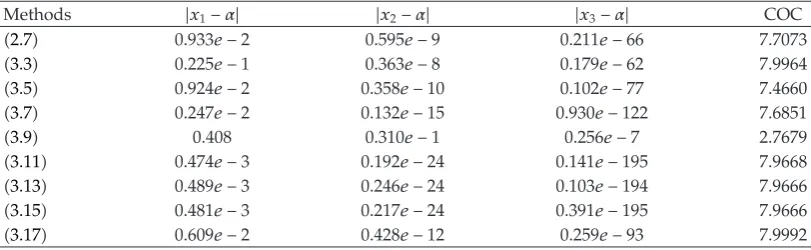
Table 5: Errors occurring in the estimates of the root of4.5by the methods described.
Methods |x1−α| |x2−α| |x3−α| COC
2.7 0.933e−2 0.595e−9 0.211e−66 7.7073
3.3 0.225e−1 0.363e−8 0.179e−62 7.9964
3.5 0.924e−2 0.358e−10 0.102e−77 7.4660
3.7 0.247e−2 0.132e−15 0.930e−122 7.6851
3.9 0.408 0.310e−1 0.256e−7 2.7679
3.11 0.474e−3 0.192e−24 0.141e−195 7.9668
3.13 0.489e−3 0.246e−24 0.103e−194 7.9666
3.15 0.481e−3 0.217e−24 0.391e−195 7.9666
3.17 0.609e−2 0.428e−12 0.259e−93 7.9992
and the exact value of the simple root of4.4isα−1. InTable 4are the errors obtained by each of the methods described, based on the initial approximationx0−2−1.
4.5. Numerical Example 5
In this subsection, we take another nonlinear equation. We will demonstrate the convergence of the new eighth-order derivative-free methods for the following nonlinear equation:
fx x11 x 1, 4.5
and the exact value of the simple root of4.5isα −0.8443975. . .. InTable 5are the errors obtained by each of the methods described, based on the initial approximationx0−1.
4.6. Numerical Example 6
In the last but not least of the examples, we take another different type of nonlinear equation. We will demonstrate the convergence of new eighth-order derivative-free methods for the following nonlinear equation:
[image:11.600.97.503.269.394.2]Table 6: Errors occurring in the estimates of the root of4.6by the methods described.
Methods |x1−α| |x2−α| |x3−α| COC
2.7 0.320e−2 0.116e−10 0.114e−75 7.5078
3.3 0.778e−2 0.270e−12 0.725e−96 7.9904
3.5 1.43 — — —
3.7 0.282 — — —
3.9 0.119e−2 0.568e−19 0.153e−149 7.7503
3.11 0.790e−3 0.193e−20 0.250e−161 7.9997
3.13 0.115e−2 0.390e−19 0.693e−151 7.9996
3.15 0.957e−3 0.896e−20 0.535e−156 7.9997
3.17 — — — —
and the exact value of the simple root of4.6isα 2. InTable 6are the errors obtained by each of the methods described, based on the initial approximationx01.9.
5. Remarks and Conclusion
We have demonstrated the performance of a new family of eighth-order derivative-free methods. Convergence analysis proves that the new methods preserve their order of convergence. There are two major advantages of the eighth-order derivative-free methods. Firstly, we do not have to evaluate the derivative of the functions; therefore, they are especially efficient where the computational cost of the derivative is expensive, and secondly we have established a higher order of convergence method than the existing derivative-free methods 6, 7. We have examined the effectiveness of the new derivative-free methods by showing the accuracy of the simple root of a nonlinear equation. The main purpose of demonstrating the new eighth-order methods for six types of nonlinear equations was purely to illustrate the accuracy of the approximate solution and the computational order of convergence.
References
1 S. D. Conte and C. de Boor, Elementary Numerical Analysis: An Algorithmic Approach, McGraw-Hill Book, New York, NY, USA, 1981.
2 J. F. Steffensen, “Remark on iteration,” Skandinavisk Aktuarietidskrift, vol. 16, pp. 64–72, 1933.
3 W. Bi, H. Ren, and Q. Wu, “A new family of eighth-order iterative methods for solving nonlinear equations,” Applied Mathematics and Computation, vol. 214, no. 1, pp. 236–245, 2009.
4 J. R. Sharma and R. Sharma, “A new family of modified Ostrowski’s methods with accelerated eighth order convergence,” Numerical Algorithms, vol. 54, no. 4, pp. 445–458, 2010.
5 R. Thukral, “A new eighth-order iterative method for solving nonlinear equations,” Applied
Mathematics and Computation, vol. 217, no. 1, pp. 222–229, 2010.
6 A. Cordero, J. L. Hueso, E. Martinez, and J. R. Torregrosa, “Steffensen type methods for solving nonlinear equations,” Applied Mathematics and Computation, vol. 194, no. 2, pp. 527–533, 2007. 7 S. K. Khattri and I. K. Argyros, “Sixth order derivative free family of iterative methods,” Applied
Mathematics and Computation, vol. 217, no. 12, pp. 5500–5507, 2011.
8 S. Weerakoon and T. G. I. Fernando, “A variant of Newton’s method with accelerated third-order convergence,” Applied Mathematics Letters, vol. 13, no. 8, pp. 87–93, 2000.
9 W. Gautschi, Numerical Analysis: An Introduction, Birkh¨auser, Boston, Mass, USA, 1997.
10 J. F. Traub, Iterative Methods for Solution of Equations, Chelsea Publishing, New York, NY, USA, 1977. 11 H. T. Kung and J. F. Traub, “Optimal order of one-point and multipoint iteration,” Journal of the
Submit your manuscripts at
http://www.hindawi.com
Hindawi Publishing Corporation
http://www.hindawi.com Volume 2014
Mathematics
Journal ofHindawi Publishing Corporation
http://www.hindawi.com Volume 2014
Hindawi Publishing Corporation http://www.hindawi.com
Differential Equations International Journal of
Volume 2014
Applied MathematicsJournal of
Hindawi Publishing Corporation
http://www.hindawi.com Volume 2014
Hindawi Publishing Corporation
http://www.hindawi.com Volume 2014
Hindawi Publishing Corporation
http://www.hindawi.com Volume 2014
Mathematical PhysicsAdvances in
Complex Analysis
Journal ofHindawi Publishing Corporation
http://www.hindawi.com Volume 2014
Optimization
Journal ofHindawi Publishing Corporation
http://www.hindawi.com Volume 2014
Combinatorics
Hindawi Publishing Corporation
http://www.hindawi.com Volume 2014
International Journal of
Hindawi Publishing Corporation
http://www.hindawi.com Volume 2014
Journal of
Hindawi Publishing Corporation
http://www.hindawi.com Volume 2014
Function Spaces
Abstract and Applied Analysis
Hindawi Publishing Corporation
http://www.hindawi.com Volume 2014
International Journal of Mathematics and Mathematical Sciences
Hindawi Publishing Corporation http://www.hindawi.com Volume 2014
The Scientific
World Journal
Hindawi Publishing Corporationhttp://www.hindawi.com Volume 2014
Hindawi Publishing Corporation
http://www.hindawi.com Volume 2014
Discrete Dynamics in Nature and Society
Hindawi Publishing Corporation
http://www.hindawi.com Volume 2014
Hindawi Publishing Corporation
http://www.hindawi.com Volume 2014
Discrete Mathematics
Journal ofHindawi Publishing Corporation
http://www.hindawi.com Volume 2014
Hindawi Publishing Corporation
http://www.hindawi.com Volume 2014