A Distributed Energy-Efficient Target Tracking Protocol
for
Three Level Heterogeneous Sensor Networks
Yashveer Singh
Department of ComputerScience Sunder Deep College of Engineering Technology,
Ghaziabad, India
Samayveer Singh,
Division of ComputerEngineering Netaji Subhas Institute of Technology, New Delhi, India
Rajeev Kumar
Division of ComputerEngineering Netaji Subhash Institute of Technology, New Delhi, India
ABSTRACT
In this paper, a distributed energy-efficient target tracking protocol for three levels heterogeneous wireless sensor networks have been reported. We have proposed heterogeneous distributed algorithm HADEEPS, based on the scheduling and adjustable range that allow sensor nodes to go into different states. Here, three types of sensor nodes i.e super, advance and normal nodes are used in our simulated network. These sensor nodes used through a heterogeneity model that directly impact on the battery power of sensor nodes and shuffling the cover set over time. The simulation results for target tracking protocol HADEEPS verify that the overall network lifetime significantly improved as compared with existing protocols. Lifetime of the network increases with three level heterogeneity because energy consumption is low as compare to homogeneous.
Keywords
: Wireless sensor networks,energy-efficiency, lifetime, sensor nodes, adjustable sensing range.
1. INTRODUCTION
WSN is distributed and centralized system, in which a large number of little and inexpensive devices, sometimes called Motes or sensor nodes are deployed. The sensor nodes collect and aggregate data from the environment via multiple hops relaying. Wireless sensor networks are a facilitator for different applications: sound, vibrations, pressure, temperature, agricultural, medical, habitat monitoring, military surveillance and environmental. Sensor networks bridge the gap between the physical and computational world by allowing the reliable, scalable, fault tolerant and precise monitoring of the physical phenomenon.
A node of the WSN consists of the battery, a radio transceiver with an internal antenna or connection to an external antenna, sensing hardware and embedded processor and memory. Traditional ad hoc networks are limited in memory, energy and computational capacity in contrast to WSNs. An important issue in sensor networks is power scarcity, driven in part by battery size and weight limitations. Mechanisms that optimize sensor
energy utilization have a great impact on prolonging the sensor network lifetime [1]. Power saving mechanism can be classified into two ways: adjusting the transmission or sensing range and scheduling the sensor nodes. In this power saving mechanism, makes cover sets and change sensor nodes
Positions i.e alternate between active and sleep modes [2, 3, 4].
In this paper, sensor network is consisting with heterogeneous nodes which are deployed in an effective and efficient manner to increasing the network lifetime. We perform operation on a heterogeneous sensor network with three types of nodes such as normal, advance and super nodes. They can be going into ideal, sleep and deciding states [5, 6, 7]. These heterogeneous sensor nodes deployed with some fraction in the monitoring resign. Advance nodes and super nodes are equipped with more battery energy than normal nodes. According this model, we have proposed HADEEPS, protocol with adjustable range, scheduling and heterogeneous model that significantly increases the lifetime of the network. Our simulation results show HADEEPS provide longer lifetime than existing protocols. This network works until, if there is a target which is not covered by any cover-sets. Whenever in this network a single target is not covered by any sensor then networks fail and finally calculate the overall lifetime of sensor networks.
The remainder of the paper is prepared as follows: In Section 2, we present some related work. In Section 3, we discuss network model. In Section 4, we provide details of distributed algorithms for SNLP and its simulation. We present results and discussion in Section 5. The paper has been concluded in Section 6.
2. RELATED WORK
with its neighbors with in a fixed ranges and adjustable sensing range.
In[1], investigate a problem of maximizing the lifetime for which the network meets its target coverage objective. In this a subset of sensors need to be in “sense” or “active” mode at any given time to meet the target coverage objective, while others can go into a power conserving “sleep” mode and these active set of sensors is known as a cover sets. The lifetime of the sensor network can be extended by shuffling the cover set over time.
M. Cardei at el [2] propose the adjustable sensing range set-cover problem and objective of that problem is to finding a maximum number of cover sets and adjustable ranges for all the targets. Sensor can be participated in multiple cover sets but the energy spent in every cover sets are constrained by the initial energy resources.
In [5, 6, 7] we have studied three type of nodes heterogeneity i.e super, advance and normal nodes and implemented that node heterogeneity in target-supervising algorithm.
In [8] the authors introduce energy efficient data gathering structure to represent the monitoring area, efficiently provable centralized algorithms for sensor monitoring schedule increasing the lifetime and a family of energy efficient distributed protocol with trade-off between communication and monitoring power consumption. In [3] authors propose distributed energy-efficient protocols for target-monitoring and sensing and using LEACH protocol for data delivery to the base-station as a communication protocol.
In [9] propose a distributed algorithmic framework for coverage problems in wireless sensor networks. It is an extension of distributed algorithms in [10] with a distributed algorithmic framework to enable sensors to determine their sleep-sense cycles based on specific coverage goals. Their approach differs from [10] in that they focus on the coverage problem whereas [10] focuses based on dependencies among cover sets.
In [12], the authors initiate algorithms where each sensor can generate a number of schedules which are exchanged with the neighbouring sensors and the most appropriate scheduled is then selected. These algorithms are analyzed through simulations.
3. NETWORK MODEL
This network model is similar to the models described in [1, 3, 4, 8, 11]. We assume that sensor nodes are deployed over the monitored region R and each sensor knows its sensor IDs, initial battery power and its own coordinates as well as coordinates of all the covered targets. Each sensor node S has its own monitoring targets T where S can collect the information for the monitoring target T without the help of any other sensor. In this network model, a sensor node is either in the communication mode or monitoring mode.
In overall communication a sensor can either be in the sleeping, listening, receiving, sending state and during monitoring, it can either be in the idle state or active state as in [10]. For saving the energy we also assume that
number of sensors go to beyond limit the number of targets need to monitor so that some sensors can turn themselves into sleep mode or some turn into active state with adjustable sensing range. We also consider that each sensor can broadcast just before the battery exhaustion so that neighboring sleep node can wake up to replace the exhausted sensor.
Given a targeted region R, a set of sensor nodes S1,
S2,..., Sm and a set of targets T1,T2,..., Tn and energy supply bi for each sensor node, find a monitoring schedule (C1, t1), (C2, t2), ………, (Ck, tk) and a range assignment for each sensor in a set Ci such that
a. t1 + t2 + ……. + tk is maximized,
b. each set cover monitors all target T1,T2,..., Tnand c. each sensor Si does not appear in the set C1… Ck for a time more than bi where bi is the initial energy of sensor of Si.
4. DISTRIBUTED ALGORITHM FOR
SNLP AND ITS SIMULATION
In this section first, we have discussed heterogeneous distributed algorithm after that we present
simulation
steps for HADEEPS.
4.1
HETEROGENEOUS
DISTRIBUTED
ENERGY
EFFICIENT
PROTOCOL
FOR
ADJUSTABLE RANGE SENSING (HADEEPS)
In this section HADEEPS protocol has been characterized for heterogeneity and adjustable sensing range.
In this network, Sensor nodes are divided into three categories such as advance, super and normal nodes. These sensor nodes used through a heterogeneity model that directly impact on the battery power of sensor nodes. In the HADEEPS each sensor at any moment is in one of three states i.e active, idle and deciding states.
active state: the sensor is active and monitors the all targets
idle state: In idle state sensor listens to other sensors, but does not monitor targets
deciding state: the sensor node monitors targets, but will alter its state to either active or idle state soon In this algorithm, which targets will be sinks and hills have been decided by us before defining the transition rules and for each target T at least one sensor placed as an in-charge.
The description of lifetime of a sensor and maximum lifetime of a target as follows.
Let Lt (b, r, e) be the lifetime of a sensor, here b is the battery, r is sensing range where r ≤ maximum sensing range and e is the energy mode. Then, the maximum lifetime of a target would be
Lt (b1, r1, e) + Lt (b2, r2, e) + Lt (b3, r3, e) + …,
assuming it can be covered by neighborhood sensors with batteries bi at a distance ri for i = 1, 2 , …
poorest in maximum lifetime for any of its covering sensors.
The following two rules decide which sensor should be in-charge of target T:
If the target is a sink, then the sensors Scovering T with the maximum lifetime Lt (b, r, e) for which Tis the poorest is positioned in-charge of T
If target Tis a hill then the largely sensors covering T the sensor S whose poorest target has the most prominent lifetime is positioned in-charge of T. If there are several such sensors, then the richest among them is positioned in-charge of T.
Various transition rules are used to change the state of sensors and when a sensor is in the deciding state with range r, its state change into active and idle.
- Active state with sensing range r, if there is a farthest target at range r less than or equal to r which is not covered by any other active or deciding sensors.
- Idle state, whenever a sensor s is not in-charge of any target except those already covered by on-sensors, S
switches itself to idle state.
Decision of all the states to be active or idle state is deciding by sensors and each sensor will stay in that state for a specified period of time called, shuffle time, or up to that time when active sensor consumes its energy supply and is going to die. Here wakeup call is used for alerting all sensors and then they change their state back to the deciding state with their maximum sensing range. Finally, the network fails if there is a target which is not covered by any sensor.
4.2 SIMULATION SETUP
For wide range of physical sensor network sizes with varying node densities this simulator is designed. The position of the sensor nodes and target can be placed randomly while creating the sensor and target inputs. For the simulation purpose, we created a network of sensors in a 100m x 100m area.
The adjustable parameters are:
The initial energy of each sensor node is 2 J. S, number of sensor nodes. We vary this from 20 to
200.
T, number of targets. We vary this to 25 and 50. P sensing ranges r1, r2,..., rP. We vary this to 30m
and 60m and each sensor has P = 2 sensing ranges with values 30m and 60m.
The energy model can be either linear or quadratic energy as defined in [6].
The linear model defined as , where the energy ep needed to cover a target at distance rp , c1
isconstant.
Quadratic model is defined as
, wherec2
is a constant.
In this paper we defined constants
E / ( ∑ ) and E / ( ∑ ), Where
E= ( ( )) is the sensor initial energy of the new heterogeneous network in [5, 6, 7].
In this paper, sensor nodes are equipped with more energy than the normal sensor nodes.
Let m be the fraction of the total number of nodes n, and mo is the percentage of the total number of nodes
m which are equipped with β times more energy than the normal nodes, we call these nodes as super nodes.
The rest ( ) nodes are equipped with times more energy than the normal nodes; we refer to these nodes as advanced nodes and remaining ( ) as normal nodes.
Suppose E0 is initial energy of each normal node. The energy of each super node is then ( ) and each advanced node is then ( ).
For algorithms, the following steps are required for the simulation:
Step:1. Generate the target and sensor files which contain the information of the target (id, position), sensor (id, initial battery, x-y axis position).
Step:2. Simulation is started from the command prompt wherein the target and sensor file, the maximum sensing range, and the energy model are provided as an input.
Step:3. Simulation is started, using these data and some other parameters.
Step:4. The simulation runs until a target cannot be covered by any cover sets.
Step:5. The simulations stops, and the overall lifetime of the network is printed out as the result.
5. RESULTS AND DISCUSSION
Case-I: m=0.2, m
0=0.5, α=2, β=1
Figure 1 (a&b) indicates the lifetime for sensor nodes in case of linear and quadratic energy model with adjustable sensing range of 50M and number of targets 25 and 50.
(a)
0 500 1000 1500
40 60 80 100 120 140 160 180 200
Li
fetim
e
(H
o
u
rs)
HADEEPS -25 Targets
ADEEPS -25 Targets
HADEEPS -50 Targets
ADEEPS-50 Targets
(b)
Figure 1 lifetime for sensor networks in case of (a) Linear Energy Model (b) Quadratic Energy Model.
The results have been obtained for modified HADEEPS and their comparison has been reported for lifetime with ADEEPS. It has been shown that the overall network lifetime significantly improved with HADEEPS in comparison of existing protocol ADEEPS in linear and quadratic energy models. It is evident from the results that for 200 numbers of sensors the lifetime obtained is [984, 694, 712, 487] and [91, 58, 72, 48] hours respectively for both energy models at the different number of targets. In case of linear and quadratic energy model with heterogeneity there is enhancement of [893, 639, 640, 439] hours in lifetime at different number of targets of a wireless sensor networks with HADEEPS protocols.
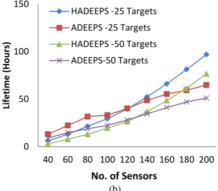
Figure 2 (a&b) mentioned the lifetime for sensor nodes in case of linear and quadratic energy model with adjustable sensing range of 100M and numbers of targets 25 and 50.
(a)
(b)
Figure 2 lifetime for sensor networks in case of (a) Linear Energy Model (b) Quadratic Energy Model.
The results have been found for modified HADEEPS and their comparison has been reported for lifetime with ADEEPS. It has been shown that the overall network lifetime significantly improved with HADEEPS in comparison of existing protocol ADEEPS in linear and quadratic energy models. It is evident from the results that for 200 numbers of sensors the lifetime obtained is [1184, 815, 799, 542] and [96, 64, 76, 51] hours respectively for both energy models at the different number of targets. In case of linear and quadratic energy model with heterogeneity there is enhancement of [1088, 751, 723, 491] hours in lifetime at different number of targets of a wireless sensor networks with HADEEPS protocols.
Case-II: m=0.2, m
0=0.5, α=1, β=2
Figure 3 (a&b) points out the lifetime for sensor nodes in case of linear and quadratic energy model with adjustable sensing range of 50M and numbers of targets 25 and 50.
(a)
0 20 40 60 80 100
40 60 80 100 120 140 160 180 200
Li
fetim
e
(H
o
u
rs)
HADEEPS -25 Targets
ADEEPS -25 Targets
HADEEPS -50 Targets
ADEEPS-50 Targets
No. of Sensors
0 500 1000 1500
40 60 80 100 120 140 160 180 200
Li
fetim
e
(H
o
u
rs)
HADEEPS -25 Targets
ADEEPS -25 Targets
HADEEPS -50 Targets
ADEEPS-50 Targets
No. of Sensors
0 50 100 150
40 60 80 100 120 140 160 180 200
Li
fetim
e
(H
o
u
rs)
HADEEPS -25 Targets ADEEPS -25 Targets
HADEEPS -50 Targets ADEEPS-50 Targets
No. of Sensors
0 500 1000
40 60 80 100 120 140 160 180 200
Li
fetim
e
(H
o
u
rs)
HADEEPS -25 Targets ADEEPS -25 Targets HADEEPS -50 Targets ADEEPS-50 Targets
[image:4.595.57.270.74.269.2](b)
Figure 3 lifetime for sensor networks in case of (a) Linear Energy Model (b) Quadratic Energy Model
.
The results have been obtained for modified HADEEPS and their comparison has been reported for lifetime with ADEEPS. It has been shown that the overall network lifetime significantly improved with HADEEPS in comparison of existing protocol ADEEPS in linear and quadratic energy models. It is evident from the results that for 200 numbers of sensors the lifetime obtained is [917, 694, 663, 487] and [85, 58, 67, 48] hours respectively for both energy models at the different number of targets. In case of linear and quadratic energy model with heterogeneity there is enhancement of [832, 636, 596, 439] hours in lifetime at number of different targets of a wireless sensor networks with HADEEPS protocols.
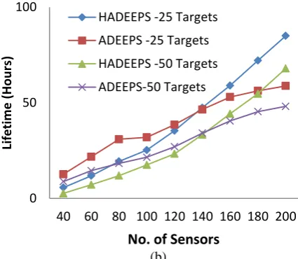
Figure 4 (a&b) suggest the lifetime for sensor nodes in case of linear and quadratic energy model with adjustable sensing range of 100M and numbers of targets 25 and 50.
(a)
[image:5.595.310.527.74.259.2](b)
Figure 4 lifetime for sensor networks in case of (a) Linear Energy Model (b) Quadratic Energy Model.
The results have been got for modified HADEEPS and their comparison has been reported for lifetime with ADEEPS. It has been shown that the overall network lifetime significantly improved with HADEEPS in comparison of existing protocol ADEEPS in linear and quadratic energy models. It is evident from the results that for 200 numbers of sensors the lifetime obtained is [1150, 815, 747, 542] and [90, 64, 70, 51] hours respectively for both energy models at the different number of targets. In case of linear and quadratic energy model with heterogeneity there is enhancement of [1060, 751, 677, 491] hours in lifetime at different number of targets of a wireless sensor networks with HADEEPS protocols.
6. CONCLUSIONS
In this paper, we have formulated a sensible networks lifetime problem and suggested a distributed algorithm for solving this problem. The distributed algorithm has tested by C++ simulations with heterogeneous networks. This distributed algorithms works at different number of targets, sensors and heterogeneity levels. The whole lifetime of the networks has been calculated when total target is covered by the cover sets during the simulation of nodes. The proposed algorithm HADEEPS is shown to be superior to the previous monitoring schedulers. Results have been reported that the overall lifetime of network 30-40% improved with HADEEPS in comparison of existing algorithms ADEEPS in linear energy model and quadratic energy model.
REFERENCES
[1] Akshaye Dhawan,“Distributed Algorithms for Maximizing the Lifetime of Wireless Sensor Networks”, Doctor of Philosophy, Dissertation Under the direction of Sushil K. Prasad, December 2009,Georgia State University,Atlanta, Ga 30303. [2] M. Cardei, J. Wu, M. Lu, Improving network lifetime
using sensors with adjustable sensing ranges, International Journal of Sensor Networks, (IJSNET), Vol. 1, No. 1/2, 2006.
0 50 100
40 60 80 100 120 140 160 180 200
Li
fetim
e
(H
o
u
rs)
HADEEPS -25 Targets
ADEEPS -25 Targets
HADEEPS -50 Targets
ADEEPS-50 Targets
No. of Sensors
0 500 1000 1500
40 60 80 100 120 140 160 180 200
Li
fetim
e
(H
o
u
rs)
HADEEPS -25 Targets ADEEPS -25 Targets HADEEPS -50 Targets ADEEPS-50 Targets
No. of Sensors
0 50 100
40 60 80 100 120 140 160 180 200
Li
fetim
e
(H
o
u
rs)
HADEEPS -25 Targets
ADEEPS -25 Targets
HADEEPS -50 Targets
ADEEPS-50 Targets
[3] Brinza, D. and Zelikovsky, A, “DEEPS: Deterministic Energy-Efficient Protocol for Sensor networks”, ACIS International Workshop on Self-Assembling Wireless Networks (SAWN'06), Proc. of SNPD, pp. 261-266, 2006.
[4] M. Cardei, J. Wu, N. Lu, M.O. Pervaiz, “Maximum Network Lifetime with Adjustable Range”, IEEE Intl. Conf. on Wireless and Mobile Computing, Networking and Communications (WiMob'05), Aug. 2005.
[5] Dilip Kumar, T. S. Aseri, R. B. Patel “EEHC: Energy efficient heterogeneous clustered scheme for wireless sensor networks”, International Journal of Computer Communications, Elsevier, 2008, 32(4): 662-667, March 2009.
[6] Yingchi Mao, Zhen Liu, Lili Zhang, Xiaofang Li, "An Effective Data Gathering Scheme in Heterogeneous Energy Wireless Sensor Networks," cse, vol. 1, pp.338-343, 2009 International Conference on Computational Science and Engineering, 2009. [7] Dilip Kumar, T. S. Aseri, R.B Patel “EECHE:
Energy-efficient cluster head election protocol for heterogeneous Wireless Sensor Networks,” in Proceedings of ACM International Conference on Computing, Communication and Control-09(ICAC3'09), Bandra, Mumbai, India, 23-24 January 2009, pp. 75-80.
[8] P. Berman, G. Calinescu, C. Shah and A. Zelikovsky, "Power Efficient Monitoring Management in Sensor Networks," IEEE Wireless Communication and Networking Conference (WCNC'04), pp. 2329-2334, Atlanta, March 2004.
[9] Akshaye Dhawan and Sushil K. Prasad. A Distributed Algorithmic Framework for Coverage Problems in Wireless Sensor Networks. In Proceedings of the 22nd IEEE Parallel and Distributed Processing Symposium, 2008.
[10] Sushil K. Prasad and Akshaye Dhawan. “Distributed Algorithms for lifetime of Wireless Sensor Networks
Based on Dependencies Among Cover Sets”. In
Proceedings of the 14th International Conference on High Performance Computing, Springer, pp. 381-392, 2007.
[11] A. Dhawan, C. T. Vu, A. Zelikovsky, Y. Li, and S. K. Prasad, “Maximum Lifetime of Sensor Networks with Adjustable Sensing Range”, 2nd ACIS International Workshop on Selfassembling Wireless Networks, (SAWN 2006), Las Vegas, NV, June 19-20, 2006. [12] M. Cardei, M.T. Thai, Y. Li, and W. Wu,
“Energy-efficient target coverage in wireless sensor networks”, In Proc. of IEEE Infocom, 2005.
[13] Samayveer Singh and Ajay K Sharma, “Energy- Efficient Data Gathering Algorithms for Improving Lifetime of WSNs with Heterogeneity and Adjustable Sensing Range”, International Journal of Computer Applications 4(2):17–21, July 2010. Published By Foundation of Computer Science.
[14] Samayveer Singh and Ajay K Sharma, “A Heterogeneous Power Efficient Load Balancing Target-Monitoring Protocol for Sensor Networks”, 2010 1st IEEE International Conference on Parallel, Distributed and Grid Computing (PDGC - 2010).