Development of Nonlinear Model and Performance
Evaluation of Model based Controller and Estimator for
the Efficient Control of Three-Tank Hybrid System
Shijoh V.
Department of Electrical Engineering NIT Calicut, Kerala, India, 673601
M. V. Vaidyan
Department of Electrical Engineering NIT Calicut, Kerala, India, 673601
ABSTRACT
In recent years researches in hybrid system dynamics and control strategies have become very prominent because most of the systems show hybrid behavior (continuous and discrete) in their dynamics. In this work authors have considered a three-tank autonomous hybrid system for the investigation. Implementation aspects of the model based control scheme and a derivative-free state estimator for three-tank hybrid system are simulated in MATLAB platform. In the simulation studies on benchmark three tank hybrid systems, the efficacy of the proposed controller and estimator under various real time operating conditions is demonstrated.
Key words
Hybrid systems, Inverse dynamics controller, State estimator, UKF Algorithm.
1.
INTRODUCTION
The dynamical systems which have both continuous and discrete behavior are termed as Hybrid systems. They demand the combination of continuous system descriptions like differential equations with discrete event models. Hybrid system arises, when the continuous and discrete dynamics interact. Mathematical models which combines the dynamics of the continuous parts of the system with the dynamics of logic and discrete part is required to capture the evolution of hybrid systems. The research of the hybrid system theory comprises of collection of modeling, analysis and controlling technique. Hybrid system theory plays an important role in the multi disciplinary design of many technological systems around us. The main sources of motivation to study hybrid system are related to (i) the design of technological systems, (ii) networked control system (iii) physical processes which exhibit non-smooth behavior.[11]
Timothy J. H. and David K. W., provide a rigorous approach to modeling, simulating and analyzing hybrid system using constraint logic programming with interval arithmetic [1]. Many
approaches are now available in the literature for control of hybrid systems based on linear hybrid models. Most of them are using linear approximations of nonlinear systems [2][3][4][5]. In this context very less work has been reported on the direct use of nonlinear models for control. Recently a novel identification method and predictive control of nonlinear hybrid system using structural approach is proposed for a class of hybrid systems by Nandola and Bhartiya [7]. Using Bayesian approach they developed a nonlinear model by combining multiple local linear models. An experimental validation of the predictive control has reported by using the developed model by Nandola and
Bhartiya [8]. J. Lygeros, C. Tomlin, and S. Sastry [9] discuss the modeling issues, local existence, uniqueness, verification techniques, stability concerns and other lyapunov like theories for hybrid systems. J. Prakash, S. C. Patwardhan, S. L. Shah[10]
recommends a state estimation scheme for an autonomous hybrid system using ensembled Kalman filter and NMPC by using estimated state values. Later they [12] extended their work to develop a nonlinear fault tolerant control of the autonomous hybrid systems by using UKF based state estimator.
Paper [6] introduces an adaptive growing and pruning radial basis function neural network for online identification of hybrid system. Identification is based on modified UKF algorithm. The procedure is online. There are two artificial neural networks which predict the levels in each tank of benchmark two tank hybrid system. Harald Brandl, Martin Weiglhofer, and Bernhard K. Aichernig [13] present a new approach for verifying the input-output conformance of two hybrid systems. Vinay A. Bavdekar and Sachin C. Patwardhan [14] proposed to identify noise covariances associated with autonomous hybrid systems from the operating data. The state estimators used for this purpose are UKF and EnKF. The problem of estimating the noise covariance matrices is formulated as a constrained optimization problem, in which a suitable objective function of the innovation sequence is minimized.
From literature survey, it is found that no work with real time platform has been reported in the field of state estimation and control of autonomous hybrid systems using nonlinear models. In this work, by using volume balance equation and conducting the experiments for finding the process parameters of the three-tank hybrid system a first principle model for the system is formulated and the performance of the model is validated for various operating regions using real time data, collected from the experimental set up. Inverse dynamics control algorithm for controlling the output variable of the three tank hybrid system and Unscented Kalman Filter based state estimator for estimating all the state variables (levels in three tanks) were applied for simulation studies. Offline validation of the UKF algorithm has been done with the collected real time data.
2.
PROCESS DESCRIPTION
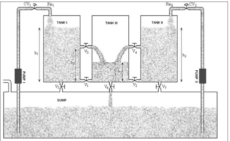
The autonomous hybrid system considered in this work for the investigation is three-tank hybrid system. The schematic representation of the three tank hybrid system is as shown in figure 1. It consists of three cylindrical tanks and a sump. Two pumps deliver water inflow, Fin1 and Fin2, to first and second
Figure 1: Schematic representation of three tank hybrid system
Tank-1 and Tank-3 as well as Tank-2 and Tank-3 are inter-connected through hand valves at two different positions. V1
and V2 are inter connecting valves at the bottom position and V3
and V4 are the intermediate interconnecting valves. Intermediate
inter connecting pipes are situated at a height of 0.3 m (h0) from
the bottom of the tank. V5, V6 and V7 are the valves in the pipes
from Tank-1, Tank-3 and Tank-2 respectively to the sump. Normally, the position of all the valves (Vi ,wherei=1, 2…7)
remain the same throughout the experiment. Flow through Vi is
denoted by Qi and corresponding discharge coefficients are
denoted by ki.
In this system, water level in the three tanks makes the continuous state, x(t) of the system and the flow through middle inter connecting pipes form the discrete state, z(t) of the system. The total height of the tank is 0.6m. An overflow is given at 0.55m height for each tank. x(t) may vary between 0 and 0.55m. The discrete state z(t)=(z1(t), z2(t)) depends on the flow through
the intermediate interconnections(Q3 and Q4).
-1 if Q3 from Tank-3 to Tank-1
z1= 0; if Q3=0
+1; if Q3 from Tank-1 to Tank-3
Similarly
-1 if Q4 from Tank-3 to Tank-2
z2= 0; if Q4=0
+1; if Q4 from Tank-2 to Tank-3
The three tank system described above is a typical hybrid system as it has both continuous and discrete states. Based on the values of continuous states the discrete states of the system is determined and based on the values of z1 and z2 , the system
may fall in to 8 different modes of operation. The continuous dynamics of the system are different under each mode. Since the automatic switching between the modes takes place based on the continuous state values, the system may classified as state driven or event driven autonomous hybrid system. The governing equations of the autonomous three-tank hybrid system are
1
1 1 1 3 5
2
2 2 2 4 7
3
3 1 2 3 4 6
dh
A =Fin -Q -Q -Q dt
dh
A =Fin -Q -Q -Q dt
dh
A =Q +Q +Q +Q -Q
dt
(1)
Where,
1
2 1 1 1 3 1 3
2 2 2 3 2 3
3 1 3 1 0 3 0
4 2 4 2 0 3 0
5 5 1 d
6 6 3 z
7 7 2 d
Q =k (h -h ) 2g h -h
Q =k (h -h ) 2g h -h
Q =z k 2g a(h -h ) b(h -h )
Q =z k 2g c(h -h ) b(h -h )
Q =k 2g(h +h )
Q =k 2g(h +h )
Q =k 2g(h +h )
sign
sign
(2)
3. METHODOLOGY
3.1 Parameter Identification
By conducting detailed study and giving a series of step changes in the two inflows, the steady state analysis is done to obtain the discharge coefficients, ki of ith valve. From these
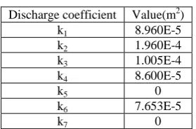
experiments, the discharge coefficients of the valves are found to be as given in Table-1.
Table 1: Discharge coefficients of the valves
Discharge coefficient Value(m2)
k1 8.960E-5
k2 1.960E-4
k3 1.005E-4
k4 8.600E-5
k5 0
k6 7.653E-5
k7 0
[image:3.595.101.241.171.263.2]The process parameter values of the three-tank hybrid system experimental setup is listed in Table-2
Table 2 : Three Tank Hybrid System Parameter Values
Parameter Value
Inner diameter of all Tanks 0.15m
Height of all Tank 0.60m
Over flow height of all tanks 0.55m Orifice diameter of tanks 0.0125m Inner diameter of all inter connecting pipes 0.0125m
Pump power rating 0.5 HP
Valve coefficients of control valves 2 Maximum rated flow rate for control valves 750 lph
3.2 Model Validation
Once the model parameters are ready, next to validate the performance of the model formulated. To validate the model, a sequence of step changes in the two inflows to the actual system is given and the response is recorded. The same input sequence is given to the model developed and compared the performance of both.
3.3 Controller and Estimation Techniques
After offline validation of the model developed using real time data, this model is used for designing a nonlinear inverse dynamics controller for controlling the output variable of the system and a UKF based state estimator for estimating all the states including non measurable states.3.3.1 Inverse Dynamics Controller Algorithm
One of the Inflows (Fin1) can be manipulated for controlling theoutput level. Other inflow (Fin2) is treated as the disturbance
variable. The control law is
1
1 in 3 3sp 3 6 3 4
dh
F =A C h -h +Q -Q -Q A1
dt
(3)
C is the tuning parameter of the controller.
3.3.2 Unscented Kalman Filter
Algorithm
All the measurable and non-measurable states are estimated using a nonlinear state estimator which makes use of Unscented Kalman Filter algorithm. Apart from Extended Kalman Filter, UKF does not require the Jacobian of the system. Therefore this algorithm is a derivative free estimation algorithm.
Unscented Kalman Filter uses unscented transformation, which is a new novel method for calculating the statistics of a random variable which undergoes a nonlinear transformation. The
n-dimensional state variable x with mean,
ˆx
k-1 and covariance,k-1
ˆP is approximated by 2n+1 weighted points called sigma points. Where n is the number of states under consideration of the process. Sigma points can be generated using the formulae given in eqn. 4. We have to assume the initial values of state variables and co variance from the available information.
(0) k-1
ˆ
x
x
(4.a)(i)
k-1 ˆk-1
ˆ
x x (n+λ)P
(4.b)
Where i=1,2,…,2n and
2
λ=α (n+κ)-n (4.c)
The constant,
α
determines the spread of the sigma points aroundˆx
k-1usually set to 1e-3 ≤ α ≤1 andκ
is secondary scaling parameter. It is usually setκ
to 0 for state estimation and to (3 – n) for parameter estimation. β is used to incorporate the prior knowledge of distribution of state. Optimum value of β is 2 for Gaussian distribution. Associated weights are computed as per equation 5.(i) (i)
m C
1
= =
2(n+λ)
W
W
(5.a)m(0) W =λ/(n+λ) (5.b) (0) C 2 λ
W = +(1-α +β)
(n+λ) (5.c)
After calculating the sigma points, time update is done as follows (eqn.6).
(i) (i)
F( , )
k-1 k-1 k/k-1
x
x
u
(6.a)
(i) (i) k/k-1 H k/k-1
z
x
(6.b) (i) (i) Wm k/k-1 k/k-1
2n
x
x
i=0
%
(6.c)2n (i) (i) W
k/k-1 m k/k-1
i=0
z
%
z
(6.d)
C
T 2 (i) (i) (i)
-
-k k/k-1 k/k-1 k/k-1 k/k-1 i=0
P
nW
x
x
x
x
Q
%
%
%
(6.e)
Measurement update equations are given in equation 7.
T zz
k k k
k
=
-ˆP P K P K
%
(7.a)k
k
k
k
k
ˆx =x +K (z -z )
%
%
(7.b) where
K
k
P P
xz zz-1(7.c) T
2
(i) (i)
(i)
zz C k/k-1 k/k-1
k/k-1 k/k-1
i=0
-
-P
nW
z
z
z
z
R
%
%
(7.d) T 2 (i) (i) (i) Wxz C k/k-1 k/k-1 k/k-1 k/k-1 i=0
-
-P
n x
x
z
z
%
%
(7.e)
4. RESULTS AND ANALYSIS
4.1 Model validation
[image:4.595.311.533.70.300.2]In this work, after developing the nonlinear model, offline validation of the model using the data collected from real-time set up has been carried out. The response shown in the figure 2 reveals that the nonlinear model developed is good enough to cope up with the all dynamics of the actual three-tank hybrid system. The input variables are tabulated in table-3.
Figure 2: Offline Model Validation using data collected from experimental setup
Table 3: Input Sequence
Sampling Instants
1-2000
2001-4000
4001-6000
6001-8000
8001-10000 Fin1 (lph) 150 375 375 150 150
Fin2 (lph) 150 150 375 375 150
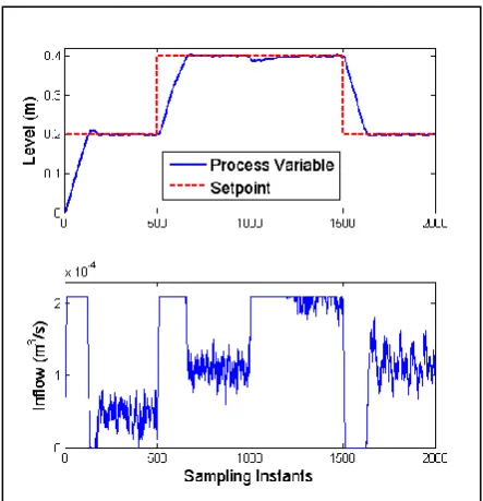
4.2 Performance of Controller
[image:4.595.59.278.181.395.2]The stability in controlling the output variable of the system under three different conditions has been investigated. The three conditions are operation below, above the intermediate connection and crossing the intermediate connection. From the figure 3, it is clear that the controller designed has very good set point tracking capability. The settling time and the integral square error are considered as the performance measure for the tuning of the controller by varying the controller gain and are tabulated in Table 4. Also a disturbance is given to the third tank level by increasing outflow from the third tank at 1000th sampling instant and the result shows that the controller designed has good disturbance rejection property.
Table 4: Tuning of IDC
Gain ISE Settling Time
.1 3.0917 150
.2 3.0889 140
.4 3.0870 97
.7 3.1193 104
1 3.1546 105
1.5 3.2335 105
Figure 3: Performance of the Inverse Dynamics Controller
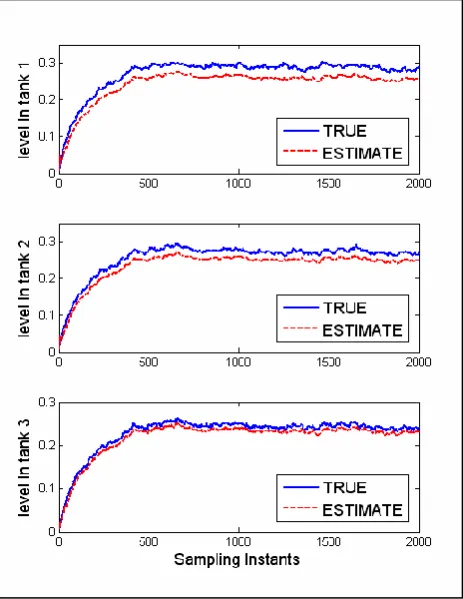
4.3. State Estimator
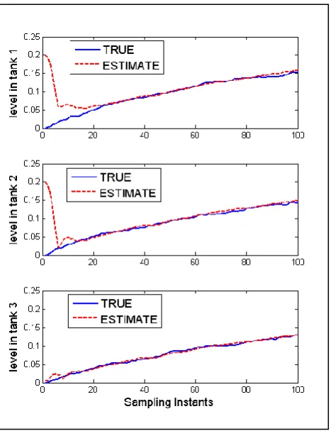
[image:4.595.321.531.471.728.2]In this work authors have assumed that only one of the three levels is available for measurement using which the other two levels are estimating using a UKF based state estimator [10]. The performance was improved by tuning the estimator by varying the process noise covariance used in the UKF algorithm.The estimator is able to predict the states of the hybrid system satisfactorily and the performance is compared with the actual level and is given in figure-4. Offline validation of the proposed estimator using the collected data has been done and the result is given in figure-5. The ISE as well as the prediction time are considered as the performance measure of the estimator and given in Table-5.
[image:4.595.102.240.601.710.2]Figure 5: Offline Validation of State Estimator
Table 5: Performance measure of UKF based estimator Gain Simulation Validation
ISE1 0.1678 –
ISE2 0.1242 –
ISE3 0.0603 0.0003
Est. Time 0.1346 0.2773
Some real-time operating constraints are introduced in the simulation and the stability of the estimator is evaluated. Figure 6 and figure 7 gives the sample graphs for the performance of the proposed estimator under model process parameter mismatch and initial condition mismatch. The proposed estimator is able to accommodate these operating condition variations. As the magnitude of mismatch in parameter value increases, estimator gives a biased estimate and the value of ISE increases as given in Table 6. Since the levels in first and second tanks are not measurable, we assumes the initial values of these two to any value which need not be the same as the original. Even if the mismatch is given in the initial state vector the estimated states are able to track the actual states within a few sampling instants. These results show the robustness of the estimator under these uncertainties.
Table 6: Performance measure of estimator with process-model parameter mismatch
Condition ISE1 ISE2 ISE3
Am= Ap, km=kp 0.0236 0.0204 0.0124
Am= 1.2Ap, km=1.2kp 0.1164 0.0981 0.0523
Am= 1.5Ap, km=1.5kp 0.3804 0.3270 0.1629
Am= 2Ap, km=2kp 0.8045 0.6950 0.3448
[image:5.595.96.247.269.355.2]Am= .8Ap, km=.8kp 0.3665 0.3168 0.0556
Figure 6.a: Performance of Estimator under process-model parameter mismatched condition (mismatch factor =1.2)
Figure 6.b: Performance of Estimator under process-model parameter mismatched condition (mismatch factor =2)
[image:5.595.313.545.419.719.2] [image:5.595.58.287.558.667.2]Figure 7: Performance of estimator under initial condition mismatch
5. CONCLUSION
The nonlinear model developed is validated using the data collectd from tha actual experimental setup. The model is able to cope up with the input variations in different modes of its operation. In order to investigate the closed loop performance, the IDC is implemented in simulatiion whose result shows that it has good servo and regulatory performance. The UKF based estimator developed for estimating the unmeasurable internal states of the system gives a very good performance under various real time operating conditions. Estimator gives the consistent performance with the realtime data collected from the experimental setup.
Further this work can be extended to the online implimentation and validation of the model as well as the controlling and estimating algorithms. Also the possibility of estimator based controller can be investigated so that all the levels can be controlled with only one measurement.
7. ACKNOWLEDGEMENT
The authors would like to thank Dr. J. Prakash, proffessor and head of the instrumentation engineering department, MIT Campus, Anna Uvniversity, Chennai for his valuable suggestions and Ideas and the permission to utilize the three tank hybrid system experimental set up present in the department for carrying out the real time data collection.
7. REFERENCES
[1] Timothy J. Hickey and David K. Wittenberg, ‘Rigorous modeling of hybrid systems using interval arithmetic constraints’, HSCC’04, 402-416, 2004.
[2] B. De Schutter, ‘Optimal control of a class of linear hybrid systems with saturation’, SIAM J. Control Opt. 39 (3) (2000) 835–851.
[3] B. Potocnik, A. Bemporad, F.D. Torrisi, G. Music, B. Zupancic, ‘Hybrid modelling and optimal control of a multiproduct batch plant’, Control Eng. Pract. 12 (9) (2004) 1127–1137.
[4] J. Thomas, D. Dumur, J. Buisson, Predictive control of hybrid systems under multi-MLD formalism with state space polyhedral partition, Proc. Am. Control Conf. (2004).
[5] F.D. Torrisi, A. Bemporad, D. Mignone, HYSDEL—A Tool for Generating Hybrid Models, Tech. Re AUT00-03, Automatic Control Lab, Swiss Federal Institute of Technology (ETH), Zurich, Switzerland, 2000.
[6] Tohid Alizadeh1, Karim Salahshoor, Mohammad Reza Jafari, Abdollah Alizadeh4, Mehdi Gholami, ‘On-line Identification of Hybrid Systems Using an Adaptive Growing and Pruning RBF Neural Network’, 1-4244-0826-1/07/$20.00 © 2007 IEEE.
[7] Naresh N. Nandola, Sharad Bhartiya, ‘A multiple model approach for predictive control of nonlinear hybrid systems’, doi:10.1016/journal of process control.2007.07.003.
[8] Naresh N. Nandola, Sharad Bhartiya, ‘Hybrid system identification using a structural approach and its model based control: An experimental validation’, Nonlinear Analysis: Hybrid Systems 3 (2009) 87_100, 1751-570X/$ _ see front matter ' 2008 Elsevier Ltd.
[9] John Lygeros, Claire Tomlin, and Shankar Sastry, ‘Hybrid Systems: Modeling, Analysis and Control’, December 28, 2008
[10] J. Prakash, Sachin C. Patwardhan, Sirish L. Shah, ‘Control of an Autonomous Hybrid System Using a Nonlinear Model Predictive Controller’, Proceedings of the 17th World Congress The International Federation of Automatic Control Seoul, Korea, July 6-11, 2008.
[11] W. P. M. H. Heemels, D. Lehmann, J. Lunze, B. De Schutter, ‘introduction to hybrid systems’, cambridge university press, 2009, 3-30.
[12] J. Prakash, Sachin C. Patwardhan, Sirish L. Shah, ‘Design and Implementation Fault Tolerant Model Predictive Control Scheme on a Simulated Model of Three-Tank Hybrid System’, 2010 Conference on Control and Fault Tolerant Systems Nice, France, October 6-8, 2010, 978-1-4244-8154-5/10/$26.00 ©2010 IEEE.
[13] Harald Brandl, Martin Weiglhofer, and Bernhard K. Aichernig, ‘Automated Conformance Verification of Hybrid Systems’, 10th International Conference on Quality Software, 1550-6002/10 $26.00 © 2010 IEEE DOI 10.1109/QSIC.2010.53
[14] Vinay A. Bavdekar, Sachin C. Patwardhan,’Identification of Noise Covariances for State Estimation of Autonomous Hybrid Systems’, 18th IFAC World Congress proceedings,9097-9102, Milano (Italy) August 28 - September 2, 2011.