4132
A NEW APPROACH FOR
MEASURING SEMANTIC
SIMILARITY OF ONTOLOGY CONCEPTS USING DYNAMIC
PROGRAMMING
1ABDELHADI DAOUI, 2NOREDDINE GHERABI AND 3ABDERRAHIM MARZOUK
13Hassan 1st University, FSTS,,IR2M Laboratory, Settat, Morocco 2Hassan 1st University, ENSAK, LIPOSI Laboratory, Khouribga, Morocco
E-mail: 1[email protected], 2[email protected], 3[email protected]
ABSTRACT
Today, with the emergence of semantic web technologies and increasing of information quantity, searching for information based on the semantic web has become a fertile area of research. For this reason, a large number of studies are performed based on the measure of semantic similarity. Therefore, in this paper, we propose a new method of semantic similarity measuring which uses the dynamic programming to compute the semantic distance between any two concepts defined in the same hierarchy of ontology. Then, we base on this result to compute the semantic similarity. Finally, we present an experimental comparison between our method and other methods of similarity measuring. Where we will show the limits of these methods and how we avoid them with our method. This one bases on a function of weight allocation, which allows finding different rate of semantic similarity between a given concept and two other sibling concepts which is impossible using the other methods.
Keywords: Semantic Web, Ontologies, Similarity Measuring, Dynamic Programming, Semantic Similarity, Semantic Distance.
1. INTRODUCTION
Recently, with explosion of information quantity in the web and the richness of natural languages used during the redaction of this information, the traditional search based on keywords has become useless (does not meet the needs of Internet users because the result depends on the keywords chosen by Internet users themselves). Therefore, a new type of search which is based on the semantic web [1] has become a necessity. Thus, the search engines that want to implement this new type of search should be able to measure the semantic similarity. For this reason, the semantic similarity measuring has become a fertile domain of research.
In this paper, our work focuses on semantic similarity measuring between concepts of ontology. This concept is a base of several works of research. The authors of [2] propose a method to compute the semantic similarity between words using a multiple information resources (lexical, corpus and taxonomy). Jeffrey Hau, William Lee
and John Darlington in [3] present a method to define the compatibility between semantic web services [4] [5] which are annotated by OWL ontologies (Web Ontology language [6]) using the semantic similarity. Also, we can find this type of measure between ontologies [7] [8], for example the authors of [8] propose a new method that allows computing the semantic similarity between two ontologies in three steps. In the first step, the authors compute the semantic similarity between the nodes of the two ontologies. Then, they compute the semantic similarity between the relations of the two ontologies. At last, the authors combine these two previous results to form one unified value which represents the semantic similarity computed between these two ontologies.
4133 these two nodes. In [9] the authors base on the same technique (dynamic programming) for computing the rate of similarity between outlines of 2D shapes using the extraction of XML data which represent local and global features of these outlines. Also, Pelin Dogan, Markus Gross and Jean-Charles Bazin in [10] have used the dynamic programming technique for temporal aligning of video frames with narrative sentences (the descriptions of natural language accompanying these videos). To do that, the authors relied on textual and visual information that provides automatic timestamps for each narrative sentence.
The current method is designed to be able to detect the small difference in the rate of semantic similarity between a given concept and two other sibling concepts defined in the same hierarchy of ontology, which is missed in the other methods of semantic similarity measurement, already exist in the literature [11] [12] [13].
The rest of the current paper is organized as follows: section 2 presents our method. Then, section 3 provides the experimental comparison with some other methods of similarity measuring. Finally, section 4 is devoted to our conclusion.
2. PROPOSED METHOD
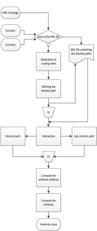
For computing the semantic similarity between two concepts present in the same hierarchy of ontology, we have designed a new method which is summarized in figure 1. This method supports the ontologies which use only the relations of type “is-a” (inheritance). Therefore, our graph will be an oriented graph towards the root node.
[image:2.612.314.519.86.572.2]
4134
<?xml version=”1.0” encoding=”utf-8” ?> <SPaths> //the list of calculed shortest paths <SPath ID=”F”> //a shortest path from a given node to the root node
<SNode> </SNode> //the start node <Node> </Node>
<Node> </Node> .
. .
<RNode> </RNode> //the root node </SPath>
. . . </SPaths>
<!ELEMENT SPaths (SPath*)>
<!ELEMENT SPath (RNode,Node*,SNode?)> <!ELEMENT SNode (#PCDATA)>
<!ELEMENT Node (#PCDATA)> <!ELEMENT RNode (#PCDATA)> <!ATTLIST SPath id ID #REQUIRED> Our designed method allows, in the first
place, the generation of the routing table for the two concepts which we need to compute the semantic similarity between them and defining the shortest paths (section 2.1). Then, we use the dynamic programming technique to calculate the semantic distance between these two concepts (section 2.2). Finally, in section 2.3 we compute the semantic similarity between these concepts using the semantic distance calculated in the previous section.
2.1 Routing Table Generation
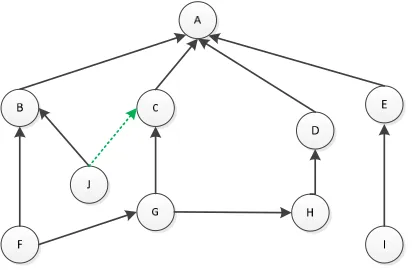
[image:3.612.314.521.317.490.2]The routing table represents a table containing the two nodes that we need to measure the semantic similarity between them and all possible paths from these nodes to the root node. We consider the following ontology:
Figure 2: An Example Of Ontology.
For example, we need to generate the routing table for the node F presented in figure 2.
Table 1: Routing Table
Nodes All paths to the root node F (F,B,A);(F,G,C,A);(F,G,H,D,A)
By analysis of this routing table, we have found three paths ((F, B, A);(F, G, C, A);(F, G, H, D, A)) between the node F and the root node. The shortest path will be the path, which has the minimum number of nodes among the generated paths in the routing table. In our example the shortest path between the node F and the root node is (F, B, A).
If we have two equal paths between the node J and the root node (figure 2), the shortest
path for the node J, which will be used, is the one that has more nodes in common with the second concept with which we want to compute the semantic similarity. For example, the shortest path for the node F is (F, B, A) and for the node J, we have two equal paths (J, B, A) and (J, C, A). But we will choose (J, B, A) because this path has more nodes in common with the concept (F, B, A) compared to (J, C, A). This technique allows minimizing the semantic distance between the concepts that we want to compute the semantic similarity between them.
To avoid redefining the shortest path for a given node more than once, we proposed to use an XML file to store the shortest paths computed for a potential use in the future. This XML file follows the structure of figure 3.
Figure 3: XML File For Storing The Shortest Paths
For validating this XML file, we use the following DTD file:
Figure 4: The Corresponding DTD File.
2.2 Semantic Distance Calculation
At this level, for computing the semantic distance between two concepts we use the dynamic programming technique to obtain the
[image:3.612.92.299.333.468.2]4135
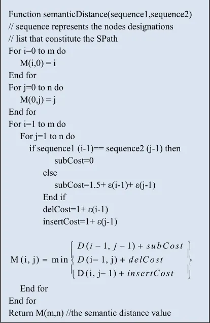
Function semanticDistance(sequence1,sequence2) // sequence represents the nodes designations // list that constitute the SPath
For i=0 to m do M(i,0) = i End for For j=0 to n do M(0,j) = j End for For i=1 to m do For j=1 to n do
if sequence1 (i-1)== sequence2 (j-1) then subCost=0
else
subCost=1.5+ ε(i-1)+ ε(j-1) End if
delCost=1+ ε(i-1) insertCost=1+ ε(j-1)
( 1, 1) M (i, j) m in (i 1, j)
D (i, j 1)
D i j subCost D delC ost
insertCost End for End for
Return M(m,n) //the semantic distance value of symbols composing the shortest path for each
of these two concepts. The value of alignment will be the semantic distance between these two concepts. In this paper, we use an algorithm of dynamic programming called Levenshtein Edit Distance [14], this algorithm allows computing the distance between two strings through a set of operations, where an operation can be a substitution, a deletion or an insertion of a single character. But we are adapting it to support execution of these three operations on a motif (node designation) that can be a single character or even a word.
Our adapted algorithm for computing the sematic distance between two concepts is designed as follows:
(i
( 1, 1)
//
(i,j) min (i 1,j) F
//adeletion
D(i,j 1) F
( 1
j )
1)
//aninserti
on
Di j
subCost asubstitution
D
D
D (i, j) represents the value of edit distance in position (i, j), F represents a fixed penalty with a value equal to one and subCost represents a cost. This cost is equal to zero if the nodes that exist in the positions (i-1) and (j-1) are identical and equal to 1.5+ ε(i-1)+ ε(j-1) if they are not identical.
1
( )
[depth(n)
(
1]
(G
n
)
)
1
N n
NTNodes
Where, ε(n) represents the weight of the node n, depth (n) represents the depth of the node n in the shortest path (the depth of the root node is equal to zero), N(n) represents the order number of this node between their siblings in the graph G (this number begins from zero). And NTNodes(G) represents the total number of nodes in the graph G.
[image:4.612.316.523.100.418.2]The formula 1 will be used for computing the matrix M[0,…,m;0,…,n], where m and n represent the length of sequences to be compared. We find the semantic distance value in M [m; n].
Figure 5: Our Adapted Algorithm For Semantic Distance Computing.
Consider the ontology presented in figure 2, if we want to compute the semantic distance between the nodes I and F, we need to define the shortest path between these nodes and the root node (in our case is A) by using the shortest path function. After execution, we obtain (A, E, I) and (A, B, F) like a result. Then, we compare these two sequences by using the dynamic programming:
Table 2: An Example of Application of Dynamic Programming Algorithm.
A E I
0 1 2 3
A 1 0 1.44 2.773
B 2 1.5 2.44 3.773 F 3 2.833 3.773 4.606 After the computation of matrix M, we can see that the semantic distance between the concepts (A, E, I) and (A, B, F) is equal to 4.606.
(1)
[image:4.612.310.526.582.659.2]4136
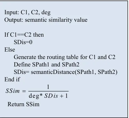
Input: C1, C2, deg
Output: semantic similarity value If C1==C2 then
SDis=0 Else
Generate the routing table for C1 and C2 Define SPath1 and SPath2
SDis= semanticDistance(SPath1, SPath2) End if
1
deg* 1
SSim
SDis
Return SSim
For minimizing the execution time of semantic distance calculation, we have designed an intermediate phase, which execute before semantic distance calculation and allows deleting the all common nodes between SPath1 and SPath2 except one node that verifies these two conditions:
1. All nodes either in SubSPath1 or SubSPath2 are connected.
2. SubSPath1 ∩ SubSPath2 = n.
Where, SPathi represents the shortest path between
a given node and the root node, SubSPathi
represents the sub shortest path of SPathi that we
find after deleting the all common nodes from SPath1 and SPath2 except the node n, which must remain in common between these two sub shortest paths.
For example, we consider the graph shown previously in figure 2. In this graph, we have the two shortest paths for the nodes J and F are (J, B, A) and (F, B, A). The computation of semantic distance on these paths is burdensome either for execution time or for memory because the calculation applied to node A is useless (especially if we have a long set of nodes in common). For this, we can use the sub shortest paths (J, B) and (F, B) in their place.
2.3 Semantic Similarity Calculation
In this section, we exploit the semantic distance computed previously in this paper to define the semantic similarity using an inverse relation between these two concepts (semantic distance and semantic similarity). By analyzing the output value of the semantic similarity function, we can categorize it in three categories:
1.The two concepts are the same. 2.Nothing in common between them. 3.There is a rate of semantic similarity
between them.
Therefore, this function should verify three conditions:
1.
, )
, , )
(
:0
(A,B) 1
2.
:
(A,A) 1
3. (
:
(A,B) SDis(A,C)then
SSim(A,B) SSim(A,C)
G
SSim
G SSim
A B
A
G if SDi
A B
C
s
Where A, B and C represent three concepts of graph G, SSim represents the semantic similarity and SDis represents the semantic distance.
To compute the semantic similarity in the current paper, we have used the function proposed in [13].
1
( , ) (0 deg 1)
deg* ( , ) 1
SSim A B
SDis A B
A and B represent two concepts that we want to compute the semantic similarity between them, the parameter “deg” represents the impact degree of Semantic distance on semantic similarity and its concrete value will be defined in the experience phase.
2.4 Global Algorithm
[image:5.612.315.522.380.570.2]Global algorithm represents the algorithm of our proposed method for computing the semantic similarity between two concepts of hierarchical ontology (all their concepts are connected by the same relation type “is-a”).
Figure 6: Our Proposed Algorithm.
3. EXPERIMENTS
This section is devoted to experimental comparison between our proposed method and two other methods of semantic similarity measuring. For this, we have used a fragment of ontology hierarchy shown in figure 7.
4137
Table 3: Computing Semantic Similarity Using [15].
Animal Bird Fish Shark Canary Ostrich Pug
Animal 1 0 0 0 0 0 0
Bird 0 1 0 0 0 0 0
Fish 0 0 1 0 0 0 0
Shark 0 0 0 1 0 0 0
Canary 0 0 0 0 1 0 0
Ostrich 0 0 0 0 0 1 0
Pug 0 0 0 0 0 0 1
Table 4: Computing Semantic Similarity Using [13].
Animal Bird Fish Shark Canary Ostrich Pug
Animal 1 0,71 0,71 0,58 0,58 0,58 0,58
Bird 0,71 1 0,55 0,47 0,76 0,76 0,47
Fish 0,71 0,55 1 0,76 0,47 0,47 0,47
Shark 0,58 0,47 0,76 1 0,41 0,41 0,41
Canary 0,58 0,76 0,47 0,41 1 0,62 0,41
Ostrich 0,58 0,76 0,47 0,41 0,62 1 0,41
Pug 0,58 0,47 0,47 0,41 0,41 0,41 1
Figure 7: A Fragment of Ontology Hierarchy.
For a better interpretation of our method, we applied the algorithm of similarity computation on the example of figure 7.
[image:6.612.91.520.248.614.2]4138 Our method is based on two steps to compute the semantic similarity.
These steps are defined as follows:
Step 1: computing the semantic distance.
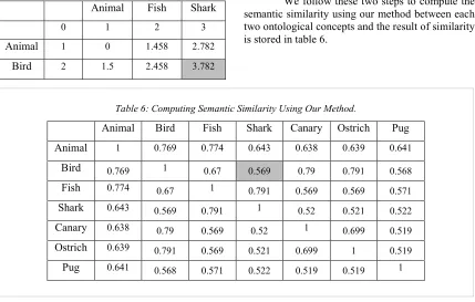
Table 5: Semantic Distance Computing Using Dynamic Programming.
Animal Fish Shark
0 1 2 3
Animal 1 0 1.458 2.782
Bird 2 1.5 2.458 3.782
Table 3 represents the results of the first method [15] which can only find the similarity between the same concepts, table 4 represents the results of the second method [13] which can find a rate of similarity between concepts of ontology as our proposed method, where our results are presented in the table 6. In contrast to our method, the method presented in table 4, gives the same rate of semantic similarity between a given concept and all the concepts, which represent a direct specification of this concept. For example the semantic similarity between the concept (Animal) and the concepts (Animal, Bird) and (Animal, Fish) is equal to 0.71. But in the reality, the semantic similarity between these concepts is different. For this reason, the rates of semantic similarity computed using our proposed method on the same concepts are different. For example, the rate of semantic similarity between (Animal) and (Animal, Bird) is equal to 0,769 and between (Animal) and (Animal, Fish) is equal to 0.774. Therefore, our method can detect even the small difference of semantic similarity rate, which resides between a
Step 2: computing the semantic similarity.
The formula for calculating the semantic similarity is defined as follows:
SSim (C1, C2)=1/(0.2*3.782+1) = 0.569 We follow these two steps to compute the semantic similarity using our method between each two ontological concepts and the result of similarity is stored in table 6.
given concept and two other sibling concepts defined in the same hierarchy of ontology which is missed in the other methods.
Also, the semantic similarity between two concepts more specific is greater than two others more generalist. For example, the semantic similarity between the concepts (Animal, Bird, Canary) and (Animal, Bird, Ostrich) is greater than the semantic similarity between (Animal, Bird) and (Animal, Fish).
In addition, we use the XML file for storing the shortest paths already computed. This technique allows minimizing the execution time that can be reserved every time for redefining these shortest paths.
[image:7.612.93.522.179.452.2]The method proposed in this paper is based on a dynamic programming algorithm, which is well known by its robustness and speed. Therefore, this one can compute the semantic similarity between concepts of hierarchical
Table 6: Computing Semantic Similarity Using Our Method.
Animal Bird Fish Shark Canary Ostrich Pug
Animal 1 0.769 0.774 0.643 0.638 0.639 0.641
Bird 0.769 1 0.67 0.569 0.79 0.791 0.568
Fish 0.774 0.67 1 0.791 0.569 0.569 0.571
Shark 0.643 0.569 0.791 1 0.52 0.521 0.522
Canary 0.638 0.79 0.569 0.52 1 0.699 0.519
Ostrich 0.639 0.791 0.569 0.521 0.699 1 0.519
4139 ontology in very short time even in industrial size ontologies.
4. CONCLUSION
In this paper, we have presented a new method for computing the semantic similarity between two concepts of the same ontology using the dynamic programming. Then, we have compared it against other methods of semantic similarity measuring and the obtained results are very interesting. These results prove that our method resolves the limitations of the other methods in some cases (where we need to compute the semantic similarity between a given concept and two other sibling concepts defined in the same ontology).
This method is not able to compute the semantic similarity between two concepts defined in two different ontologies. For this reason, in the future work, we are interested to compute the semantic similarity between concepts defined in different ontologies.
REFERENCES
[1] T. B. Lee, J. Hendler, O. Lassila, “The semantic web”, Scientific America, 2001, pp. 1-18.
[2] Y. Li, Z. A. Bandar, D. McLean, “An Approach for Measuring Semantic Similarity between Words Using Multiple Information Sources”, IEEE Transactions on Knowledge and Data Engineering, Vol. 15, No. 4, 2003, pp. 871-882.
[3] J. Hau, W. Lee, J. Darlington, “A Semantic Similarity Measure for Semantic Web Services”, the 14th international conference on World Wide Web, Chiba, Japan, 2005.
[4] M. Burstein, C. Bussler, M. Zaremba, T. Finin, M. N. Huhns, M. Paolucci, A. P. Sheth, S. Williams, “A Semantic Web Services Architecture”, IEEE Internet Computing, Vol. 9, No. 5, 2005, pp. 52-61.
[5] S. A. McIlraith, D. L. Martin, “Bringing Semantics to Web Services”, IEEE Intelligent Systems, Vol. 18, No. 1, 2003, pp. 90-93. [6] https://www.w3.org/TR/owl2-overview, last
accessed 17/11/2016.
[7] F. Li, “An Improved Method about the Similarity Calculation of Ontology”,
International Conference on Multimedia Technology, IEEE, 2010, pp. 1-4.
[8] H. Wang, X. Han, “Research on Similarity of Semantic Web”, International Conference on Computer Application and System Modeling, IEEE, 2010, pp. 166-169.
[9] N. Gherabi, M. Bahaj, “Outline Matching of the 2D Shapes Using Extracting XML Data”, ICISP 2012, Springer, Heidelberg, 2012, pp. 502–512.
[10] P. Dogan, M. Gross, J.C. Bazin, “Label-Based Automatic Alignment of Video with Narrative Sentences”. ECCV 2016, Springer International, Switzerland, 2016, pp. 605–620. [11] Z. Wu, M. Palmer, “Verb semantics and
lexical selection”, In Proceedings of the 32 Annual Meeting of the Associations for Computational Linguistics, 1994, pp. 133-138. [12] D. Lin, “An Information-Theoretic Definition
of similarity”, In Proceedings of the Fifteenth International Conference on Machine Learning. ICML 1998.
[13] J. Ge, Y. Qiu, “Concept Similarity Matching
Based on Semantic
Distance”, the 4th International Conference on Semantics, Knowledge and Grid, IEEE, 2008, pp. 380-383.
[14] E. S. Ristad, P. N. Yianilos , “ Learning String-Edit Distance”, IEEE Transactions on Pattern Analysis and Machine Intelligence, Vol. 20, No. 5, 1998,522-532.
[15] F. Giunchiglia, P. Shvaiko, M. Yatskevich ,
“S-Match: an algorithm
![Table 3: Computing Semantic Similarity Using [15].](https://thumb-us.123doks.com/thumbv2/123dok_us/8906181.956945/6.612.91.520.248.614/table-computing-semantic-similarity-using.webp)