Abstract— The Monte Carlo method is first used to estimate
the contribution of multiple scattering to acoustic signals propagating along vertical and horizontal paths in the plane-stratified moving turbulent atmosphere. Contribution of multiple scattering to sodar return signals is also analyzed. Numerical estimates are obtained as functions of sodar parameters and atmospheric conditions.
Index Terms—Monte Carlo method, atmospheric acoustics,
acoustic wave propagation, acoustic sounding
I. INTRODUCTION
ifficulties of an analytical solution of the problem of acoustic wave propagation in the atmosphere with allowance for the contribution of multiple scattering call for solving this problem by numerical methods. Here the method of statistical simulation (Monte Carlo) is most promising, because it allows multiple scattering of acoustic radiation to be correctly taken into account for realistic atmospheric models and experimental geometry.
The equation of acoustic radiation transfer in the plane-stratified turbulent moving atmosphere in the form of the Neumann series for the acoustic radiation intensity was derived in [1]. In [2], the Monte Carlo method was used to solve the problem of monochromatic acoustic radiation propagation through a 500-meter layer of the plane stratified moving turbulent atmosphere taking into account refraction of sound and statistical estimations of the contribution of multiple scattering to the distribution of the intensity of transmitted acoustic radiation over zones of the detector depending on the sound frequency and the outer scale of the atmospheric turbulence. In the present report, the Monte
Manuscript received December 8, 2015; revised February 7, 2016. This work was supported in part by the Russian Foundation for Basic Research (Grant No. 14-01-00211a, 16-01-00121a) and by the National Research Tomsk State University Academic D. I. Mendeleev Fund Program (NU 8.1.55.2015 L) in 2014-2015.
Yu. B. Burkatovskaya is with the Institute of Cybernetics, Tomsk Polytechnic University, 30, Lenin Prospect, Tomsk 634050, Russia; Department of Applied Mathematics and Cybernetics and International Laboratory of Statistics of Stochastic Processes and Quantitative Finance, Tomsk State University; 36, Lenin Prospect, Tomsk 634050, Russia (e-mail: [email protected]).
V. V. Belov is with V. E. Zuev Institute of Atmospheric Optics SB RAS; Tomsk State University, Tomsk, Russia (e-mail: [email protected]).
N. P. Krasnenko is with Institute of Monitoring of Climatic and Ecological Systems SR RAS, Tomsk State University of Control Systems and Radioelectroonic, Tomsk, Russia (e-mail: [email protected] )
L. G. Shamanaeva is with V. E. Zuev Institute of Athmospheric Optics SB RAS; Tomsk State University, Tomsk, Russia (e-mail: [email protected]).
P. A. Khaustov is with is the Institute of Cybernetics, Tomsk Polytechnic University, 30, Lenin Prospect, Tomsk 634050, Russia (e-mail [email protected]).
Carlo method is first used to estimate contribution of multiple scattering to acoustic signals propagating along vertical and horizontal paths in the plane-stratified moving turbulent atmosphere. Contribution of multiple scattering to sodar return signals is also analyzed.
II. ACOUSTIC MODEL OF THE ATMOSPHERE
For the 500-m standard plane-stratified turbulent atmosphere, the total extinction coefficient was calculated from the formula
kex(zi) = kcl+ kmol(zi) + kT(zi) + kV(zi), (1)
where kcl and kmol are the coefficients of classical and molecular absorption, kT and kV are the coefficients of
acoustic radiation scattering by atmospheric temperature and wind velocity fluctuations, zi = z(i – 1) + dz, dz = 20 m,
i = 1, …, 26, and z0 = 0. The expressions for kcl and kmol
were borrowed from [3]. In the calculation of their altitude dependence, the vertical profiles of the air temperature, pressure, and sound velocity were set according to the standard model of the atmosphere given in [4].
Analytical expressions for the volume scattering coefficients were derived in [5, 8] for the von Karman model of the three-dimensional spectra of temperature and wind velocity fluctuations:
1/3 2 2
T T
7/3 7/6 7/3
0
2 5/6 5/3
1/6 1/3 0.9
0.07143 0.1
,
i i i i
i i i
i i i
i i i
k z z C z T z
L z B z z
A z B z z
A z B z z
(2)
2/3 1/3 2
V
13/3 7/6
0
7/3 13/6 13/6
1/6 1/3
2 5/6 5/3
1.569
0.1429 2
0.0769
2
0.2 ,
i i i i
i i i i
i i i
i i i i
i i i
k z z z c z
L z B z A z B z
z B z z
A z A z B z B z z
A z B z B z z
(3)
where is the acoustic radiation wavelength, c is the velocity of sound, L0 is the outer scale of turbulence, CT2 is the structure function of the temperature field T, is the turbulent energy dissipation rate,
2 2
0 2 2 0
2 ,
4 .
i i i
i i
A z L z z
B z L z
(4)
The normalized scattering phase functions were calculated from the formulas [5]
Monte Carlo Method in Atmospheric Acoustics
Yulya B. Burkatovskaya, Vladimir V. Belov, Nikolai P. Krasnenko, Liudmila G. Shamanaeva, Pavel A.Khaustov
6 2 2
T 0 0
11/ 6
2 7 / 6
7 / 3 2 5/ 6
1
5/ 3 1/ 6 1/ 3
, 0.1062 cos 2 1
cos 0.07143
0.1
,
i i i
i i
i i i
i i i i
g z L z L z
z B z
z A z B z
z A z B z z
(5)
13/ 3 2
V 0
11/ 6 2
0
7 / 6 7 / 3 13/ 6 13/ 3
1/ 6 1/ 3
1
2 5/ 6 5/ 3
, 0.1191 cos 1 cos
/ 2 cos 0.1429
2
0.0763
2
0.2 .
i i
i i
i i i i
i i i
i i i i
i i i i
g z L z
A z L z
B z A z B z z
B z z A z
A z B z B z z
A z B z B z z
(6)
The acoustic model of the atmosphere comprised 25 layers each 20 m thick with constant within the layers coefficients of classical and molecular absorption and scattering by fluctuations of the temperature and wind velocity. The underlying surface was considered absolutely absorbing. The outer scales of the temperature (L0T) and
dynamic turbulence (L0V) were determined by the Monin–
Obukhov length LMO u T* 02 /g T * [7]:
MO0
MO
1 0.22 / /
( ) 1.3
1 0.22 /
i i
V
i
z z z L
L z z
z L
, (7)
MO
0
MO
1 7.0 /
( ) 1.5
1 10 /
T
z L
L z z
z L
, (8)
where u* is the friction velocity, T* is the surface-layer temperature scale, g is the acceleration of gravity, is the von Karman constant, Т0 is the surface temperature, and zi is
the atmospheric boundary layer height. Our calculations were performed for the unstable atmospheric stratification with light, moderate, and strong wind under conditions of cloudless (the surface flux Hs 200 W/m2) and cloudy
atmosphere (the surface heat flux Hs 40 W/m2). The
atmospheric boundary layer height zi was set equal to 1000 m. The corresponding values of the parameters u*,
*
T , and LMO for 6 meteorological regimes of the turbulence considered in [7] are given in Table 1.
TABLEI
BENCHMARK METEOROLOGICAL REGIMES OF THE UNSTABLE ATMOSPHERE
ACCORDING TO [4]
HS,W/M2 MEAN WIND
VELOCITY
U, M/S T,K LMO, M 200
LIGHT 0.1 –1.6 –0.47
MODERATE 0.3 –0.54 –13
STRONG 0.7 –0.23 –160
40
LIGHT 0.1 –0.33 –2.4
MODERATE 0.3 –0.11 –64
STRONG 0.7 –0.46 –810
As an example, Fig. 1 shows the altitude dependence of the total sound extinction coefficients (a, b) and phonon survival probabilities (c, d) for frequencies in the range 400 Hz–4 kHz and the Monin–Obukhov length LMO equal to
–0.47 m (a, c) in the cloudless atmosphere with light wind
and –810 m (b, d) in the cloudy atmosphere with strong wind. The results of calculations demonstrated that the extinction coefficient in the surface layer increased approximately by an order of magnitude, and the turbulent extinction considerably exceeded the classical and molecular absorption in the entire range of the examined frequencies (the probabilities of the phonon scattering exceeded 0.96).
10 50 90130
170 210
250290 330
370 410
450 490
10002000 30004000 0
0,5 1
Ext
h,m.
F, Hz
1000
2000
3000
4000
a
10 50 90130
170210 250
290 330
370 410
450 490
10002000 30004000 0
2,5 5
Ext
h,m.
F, Hz
1000
2000
3000
4000
b
1050 90
130 170
210 250
290 330
370 410
450 490
10002000 30004000 0,7
0,8 0,9 1
P
h,m.
F, Hz
1000 2000 3000 4000
c
10 5090
130 170
210 250
290 330
370 410
450 490
10002000 30004000 0,96
0,97 0,98 0,991
P
h,m.
F, Hz
1000 2000 3000 4000
[image:2.595.81.292.52.268.2]d
Fig. 1. Altitude dependence of the total sound extinction coefficient (a, b) and of the phonon survival probabilities (c, d) for frequencies F = 1–4 kHz and LMO = –0.47 (a, c) and –810 m (b, d).
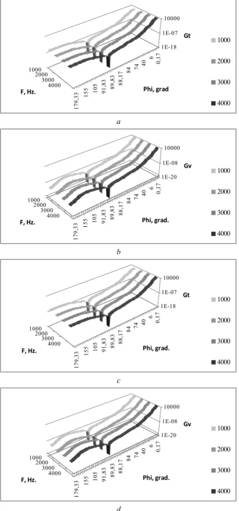
Figure 2 shows the normalized phase functions of sound scattering on the temperature (a, b) and wind velocity fluctuations (c, d) in the cloudless atmosphere with light wind for LMO = –0.47 m (a, c) and in the cloudy atmosphere
with strong wind for LMO = –810 m (b, d). It should be noted
[image:2.595.41.295.635.720.2]sound extinction coefficients and normalized phase functions of sound scattering by the atmospheric turbulence performed in [8] demonstrated their good agreement with the available experimental data.
0,
17
6
40
74
84
88
,17
89
,83
91
,83
10
5
15
5
179
,33
1000 2000
3000 4000
1E-18 1E-07 10000
Gt
Phi, grad F, Hz.
1000 2000 3000 4000
a
0,
17
6
40
74
84
88,
17
89,
83
91
,8
3
105
15
5
179,
33
1000 2000
3000 4000
1E-20 1E-08 10000
Gv
Phi, grad. F, Hz.
1000 2000 3000 4000
b
0,
17
6
40
74
84
88,
17
89,
83
91,
83
105
155
179,
33
1000 2000
3000 4000
1E-18 1E-07 10000
Gt
Phi, grad. F, Hz.
1000 2000 3000 4000
c
0,
17
6
40
74
84
88
,1
7
89
,83
91,
8
3
105
155
179,
33
1000 2000
3000 4000
1E-20 1E-08 10000
Gv
Phi, grad. F, Hz.
1000 2000 3000 4000
[image:3.595.49.290.103.618.2]d
Fig. 2. Normalized phase functions of sound scattering on the temperature (a, c) and wind velocity fluctuations (b, d) in the cloudless atmosphere with light wind for frequencies F = 1–4 kHz and LMO = –0.47 m. (a, b), LMO = – 810 m. (c, d),
III. COMPUTATIONAL ALGORITHM
The problem of acoustic radiation propagation from the source having acoustic power of 1 W with a circular aperture 1 m in diameter, beam divergence angle = 2.5– 25, and distribution density
cos2 0.12 s
R
f R A
(9)
was solved, where 0Rs 0.5 and the constant A was chosen from the normalization condition. The distribution density of the initial directional cosines of the angle with the
Oz axis was a Gaussian one. The radiation source was located on the Oz axis at the altitude Hs= 35 m above the absolutely absorbing Earth surface. Taking into account the symmetry of the problem of vertical propagation of acoustic radiation, the dependence of the transmitted and multiply scattered radiation intensity over the horizontal plane was estimated.
Acoustic radiation from the source propagated through the plane-parallel atmospheric layers with variable extinction coefficients specified by Eqs. (1)–(3). A hypothetical detector was placed above the source at an altitude of 500 m from the ground. The distribution of transmitted radiation over the horizontal plane was estimated together with the contribution of multiply scattered radiation as a function of the distance H from the vertical axis.
[image:3.595.317.536.361.744.2]Random trajectories of particles (phonons) were simulated using conventional Monte-Carlo procedures described, for example, in [9] and original procedures constructed with allowance for the specifics of the acoustic wave interaction with the atmosphere. The flowchart of the Monte Carlo algorithm is shown in Fig. 3.
Coordinates of the point of phonon emission (x0, y0, z0)
and their directional cosines (1, 2, 3) were calculated
using the procedure described in [9]. A statistical weight of the phonon = 1 after each collision decreased by e–, where is the acoustic extinction depth for the phonon moving between collision points r1 and r2:
21
r
ex r
k r dr
. (10) The phonon absorption in the medium was modeled by its annihilation, and its statistical weight was added to the element of the array determining acoustic radiation absorbed in the given atmospheric layer. The phonon free path was modeled by the following scheme.a) Let l be the distance passed by the phonon through atmospheric layers with extinction coefficient kex[1], ,
kex[N].
b) By subsequent subtraction, we find the number j of the layer such that
1
1 1
[ ] ln
j j
ex ex
m m
l k m rand l k
, (11)where rand is a random number uniformly distributed in the interval [0,1].
c) If there is no number j satisfying condition (11), it is considered that the phonon have been escaped from the medium; otherwise,
0
1 1 1
2 ln
. free
j ex m
ex
z z
l j l
c
rand l k m k j
(12)
The point of the next collision was chosen by the well-known formulas [9].
Then the collision type was chosen. The normalized absorption and scattering coefficients were calculated for each layer:
V T
V T
, ,
cl mol
abs sc sc
ex ex ex
k k k k
k k k
, (13)
and arranged in the increasing order of magnitudes. Let, for example, in the jth layer abs[ ]j scT scV. Then if rand
abs j
, the photon absorption occurred; if
j < T
abs rand sc j
, scattering by the temperature fluctuations occurred; otherwise, scattering on the wind velocity fluctuations occurred. In the case of absorption, the phonon annihilated, and its statistical weight was added to the element of the array determining the value of the acoustic energy absorbed in the jth atmospheric layer.
In the case of scattering, the scattering angle was determined by the scattering phase function given by Eq. (5) for the case of scattering by temperature fluctuations and by Eq. (6) for scattering by wind velocity fluctuations. The procedure of simulation of the angle of scattering was described in [10]. The Earth’s surface was considered absolutely absorbing, and when the phonon trajectory intersected the plane z= 0, the phonon was considered absorbed, and a new phonon history was modeled.
The propagation of nonstationary acoustic radiation in horizontal direction to a hypothetical point detector can be
described [9] by the nonstationary equation of radiation transfer of the form:
0 , ( , , ) , ( , , )
( , ) ( , ) ( , ) ( , , ) ( , )ext sc ( , )
I t grad t
с t
k I k
g I d
I
r ω ω r ω
r r ω r
r ω ω r ω ω r ω
(14)
where r is the radius vector of the point in space, is the unit vector of directions, t is time, c is the velocity of light, I
is the radiation intensity, kext is the coefficient of sound extinction at point r at the wavelength , ksc is the coefficient of sound scattering at point r at the wavelength
, is the region of variations of vectors within which multiple scattered acoustic radiation is taken into account, and and specify the directions of phonon propagation before and after scattering, g(r,) is the axisymmetric phase function of scattering between directions and , and Ф0 is the source function.
In [1] it was demonstrated that Eq. (1) can be solved by the Monte Carlo method. We performed statistical simulation of direct trajectories using the method of local estimates [2] that in the examined case has the following form for each trajectory:
, , ,
, , 2
,
( ) exp( )
2
k j k j k j
i j k i
k j
g
l
r , (15)
where k is the serial number of the next scattering point, j is the serial number of the angular receiver aperture starting from which the point rk,j remains in its field of view, i is
the indicator of the time interval (ti – ti-1) of the phonon
lifetime counted from the moment of phonon emission along the trajectory ending on the receiver through the point
rk,j, k,j is the statistical weight of the phonon that takes into
account its absorption, g(k,j) is the normalized differential scattering phase function for the angle of scattering in the direction toward the receiver from the kthscattering point,
k,j is the acoustic path length along the straight line segment
rk,j. As rk,j 0, we can neglect the divergence of estimate
(15), since there exists the so-called shadow zone from which the acoustic signal cannot be registered. In our calculations, the radius of this zone was set equal to 10 m.
Calculations were performed for 106–107 phonon
histories, which provided the standard deviation of the results obtained in the range 3–10 %.
IV. CALCULATION RESULTS AND DISCUSSION
A. Vertical Propagation Paths
direct Monte Carlo calculations with the experimental data [12] can be seen. This demonstrates the efficiency of the developed Monte Carlo algorithm.
Fig. 5. Total attenuation of acoustic waves propagating along the vertical atmospheric paths versus the distance. The solid and dashed curves here show the results of our Monte Carlo calculations; closed triangles and diamonds show results of acoustic measurements [12] with a tethered balloon.
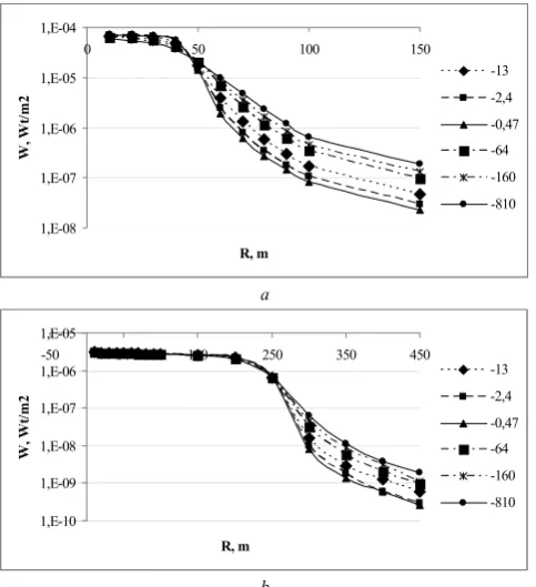
The influence of the outer scale of the atmospheric turbulence is illustrated by Fig. 6, where the distribution of the transmitted radiation intensity over the detector zones is shown for the frequency F = 1700 Hz and the angle of the source divergence of 5°.
1,E-08 1,E-07 1,E-06 1,E-05 1,E-04
0 50 100 150
R, m
W
, W
t/
m
2
-13 -2,4 -0,47 -64 -160 -810
a
1,E-10 1,E-09 1,E-08 1,E-07 1,E-06 1,E-05
-50 50 150 250 350 450
R, m
W,
Wt
/m
2
-13 -2,4 -0,47 -64 -160 -810
b
Fig. 6. Influence of the outer scale of the atmospheric turbulence on the distribution of the transmitted radiation intensity over the detector zones for the frequency F = 1700 Hz and angles of source divergence of 5° (a) and 25° (b). The Monin-Obukhov lengths are indicated on the right of the figure.
Results of our calculations demonstrated that the dependence of the transmitted radiation intensity on the source divergence angle is quadratic in character, which was also indicated in [5].
B. Horizontal Propagation
Monte Carlo calculations were also performed using the method of local estimate for near-ground paths for source altitude zs = 6 m and different detector altitudes. The source
divergence angle was 2,5. Figure 7 shows statistical estimates of the intensity of multiply scattered radiation that gives the main contribution to the signal recorded by the detector for F = 2 (a) and 3 kHz (b) for the detector located at the altitude zd = 0, 0.5, 1, and 1.5 m above the absolutely
absorbing Earth’s surface. It should be noted that the intensity of the received radiation is practically completely determined by the contribution of multiple scattering. From Fig. 7 it can also be seen that Ims = 1.5610–4 W/m2
for the 90-meter path, F = 2 kHz, and zd = 1.5 m, whereas
Ims = 7.210–5 W/m2 for the detector placed at the earth
surface, that is, it decreased by 53 %.
0 0,00004 0,00008 0,00012 0,00016
90 180 210 270
L,m
W,
Wt
/m
2 0
0,5 1 1,5
a
0 0,000001 0,000002 0,000003 0,000004 0,000005 0,000006
90 180 210 270
L,m
W,
Wt
/m
2 0
0,5 1 1,5
[image:5.595.303.544.196.470.2]b
Fig. 7. Intensities of multiply scattered radiation received by the detector at frequencies of 2 kHz (a) and 3 kHz (b) as functions of the propagation path length L for the source altitude zs = 6 m and the detector altitude zd, in m, indicated at the right of the figure.
With further increase of the propagation path length, the effect of zd decreases, and already for L = 210 m, the
difference does not exceed 7 %. For F = 3 kHz, the difference makes 39 %. The obtained statistical estimates of the singly scattered radiation intensity were compared with the results of our model calculations using the Delany– Bazley model. Results of comparison are shown in Fig. 8 for F = 1 kHz.
0 0,00005 0,0001 0,00015 0,0002 0,00025
90 140 190 240 L, m.
W,W
t/
m
2
0
1,5
[image:5.595.49.291.364.629.2] [image:5.595.307.541.617.739.2]From the figure it can be seen that for L90 m, the received signal intensity in both cases is maximum for the detector located on the earth surface. In addition, good quantitative agreement of the results is observed for this position of the detector for the propagation path lengths of 180, 210, and 270 m. They differ significantly for the 90-meter path. For zd = 1 and 1.5 m, good agreement of the
results is observed
C. Acoustic Sounding
In this report, the influence of the sodar parameters and atmospheric conditions on the contribution of multiple scattering to sodar signals is estimated with allowance for the following parameters of a monostatic sodar [6]. The frequency of sodar operation varied in the range 1–4 kHz. The angle of source divergence and the receiver field-of-view angle were in the range = 2.5–25°. The transmitted acoustic power was 1 W. Time distributions of the intensities of singly and multiply scattered sodar return signals were simulated.
0 0,02 0,04 0,06 0,08 0,1 0,12
0,
05 0,1
0,
15 0,2
0,
25
t, s
W,
w
t/
m
2
2
4
6
8
10
a
0 0,1 0,2 0,3 0,4 0,5 0,6
0,
05 0,1
0,
15 0,2
0,
25
t, s
W,
w
t/
m
2
2
4
6
8
10
b
20 30 40 50 60 70 80 90 100
0,
06 0,1
0,
14
0,
18
0,
22
0,
26 0,3
0,
34
0,
38
0,
42
0,
46 0,5
t, s
Im
s,
%
-13
-2,4
-64
-810
-160
-0,47
[image:6.595.50.285.298.705.2]c
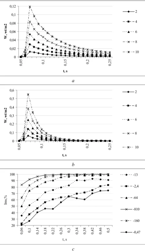
Fig. 9. Results of statistical simulation of the time histories of singly (a, b) scattered signals of the sodar operating at a frequency of 1 kHz as functions of the sodar transceiving angle (a and b) and multiply scattered sodar signal intensities as functions of the Monin-Obukhov length, in m, shown on the right of Fig. 9 c.
The calculated sodar return signals are shown in Fig. 9 a–
c for the sodar operating at F = 1 kHz under conditions of
cloudless atmosphere with LOM = –0.47 (a) and cloudy
atmosphere with LOM = –810 (b). Here the sodar
transceiving angle changed in the range = 2–20° with a step of 2°. The multiply scattered sodar signal is illustrated by Fig. 9 a and b, and Fig. 9 c shows the contribution of multiply scattered acoustic radiation as a function of the Monin–Obukhov length. The abscissa shows of signal recording time, in s, and the received signal intensity is plotted on the ordinate. It can be seen that the sodar signal is small for = 2–6°.
This allows us to conclude that for efficient operation of monostatic sodars, the transceiving angles should exceed 6°. The sodar return signal broadens with increasing sodar transceiving angle.
From Fig. 9 c it can be seen that the multiple scattering contribution is greater for cloudless atmosphere, and starting from t = 0.15 s the sodar signal is completely determined by the multiple scattering contribution. The large contribution of multiple scattering was also pointed out in [11], where it was indicated that the temperature structure characteristics retrieved from the sodar signal intensity deviated from their values measured at a must due to neglect of sodar signal scattering by the atmospheric turbulence, and the ratio of the average sodar to mast values of the temperature structure characteristics can change from 0.1 to 10 depending on the atmospheric conditions.
REFERENCES
[1] V.E. Ostashev, Sound propagation in moving media, Moscow: Nauka, 1992.
[2] V.V. Belov, Yu.B. Burkatovskaya, N.P. Krasnenko, L.G. Shamanaeva, “Statistical estimates of the influence of the angular source divergence angle on the characteristics of transmitted acoustic radiation,” Russ. Phys. J., No. 12, pp. 1264-1270, 2009.
[3] ANSI Standard S1-26-1995 (R2009), “Method for calculation of the absorption of sound by the atmosphere”.
[4] Yu. A. Glagolev, Handbook on the physical parameters of the atmosphere, Leningrad: Gidrometeoizdat, 1970.
[5] R. A. Baikalova, G. M. Krekov, L. G. Shamanaeva, “Statistical estimates of the multiple scattering contribution to sound propagation through the atmosphere”, Opt. Atm., vol. 1, No. 5, pp. 25-29, 1988. [6] N. P. Krasnenko, A.N. Kudryavtsev, E.E. Mananko, P.G. Stafeev,
“Acoustic radar “Zvuk-3” for atmospheric sounding,” Prib. Tekh. Eksper., No. 5, pp. 1-2, 2006.
[7] V.E. Ostashev, D.K. Wilson, “Relative contributions from temperature and wind velocity fluctuations to the statistical moments of a sound field in a turbulent atmosphere,” Acta Acustica United with Acustica, vol. 86, pp. 260-268, 2000.
[8] R.A. Baikalova, G.M. Krekov, L.G. Shamanaeva, “Theoretical estimates of sound scattering by atmospheric turbulence”, J. Acoust. Soc. Am., vol. 83, No. 4, pp. 1332-1335, 1988.
[9] G.I. Marchuk, G.A. Mikhailov, M.A. Nazaraliev, R.A. Darbinyan, B.A. Kargin, B.S. Elepov, Monte Carlo Method in Atmospheric Optics, Nauka, Novosibirsk, 1976.
[10] G. M. Krekov, L. G. Shamanaeva, “Statistical estimates of the spectral brightness of the twilight Earth’s atmosphere”, Atmosphric Optics,Leningrad: Gidrometeoizdat, pp. 180-186, 1974.
[11] R.L. Coulter, M.A. Kallistratova, “Two decades of progress in sodar techniques: A review of 11th ISARS Proceedings,” Meteorology and Atmospheric Physics, vol. 85, pp. 3-19, 2004.
[12] M. Aubry, F. Baudin, A. Weil, P. Rainteau, “Measurements of the total attenuation of acoustic waves in the turbulent atmosphere”, J. Geophys. Res., vol. 79, No. 36, pp. 5598–5606, 1974.