Manuscript version: Author’s Accepted Manuscript
The version presented in WRAP is the author’s accepted manuscript and may differ from the published version or Version of Record.
Persistent WRAP URL:
http://wrap.warwick.ac.uk/105574
How to cite:
Please refer to published version for the most recent bibliographic citation information. If a published version is known of, the repository item page linked to above, will contain details on accessing it.
Copyright and reuse:
The Warwick Research Archive Portal (WRAP) makes this work by researchers of the University of Warwick available open access under the following conditions.
Copyright © and all moral rights to the version of the paper presented here belong to the individual author(s) and/or other copyright owners. To the extent reasonable and
practicable the material made available in WRAP has been checked for eligibility before being made available.
Copies of full items can be used for personal research or study, educational, or not-for-profit purposes without prior permission or charge. Provided that the authors, title and full
bibliographic details are credited, a hyperlink and/or URL is given for the original metadata page and the content is not changed in any way.
Publisher’s statement:
Please refer to the repository item page, publisher’s statement section, for further information.
Multiple UAVs as Relays: Multi-hop Single
Link versus Multiple Dual-hop Links
Yunfei Chen,
Senior Member, IEEE,
Nan Zhao,
Senior Member, IEEE
,
Zhiguo Ding,
Senior Member, IEEE,
Mohamed-Slim Alouini,
Fellow, IEEE
Abstract
Unmanned aerial vehicles (UAVs) have found many important applications in communications.
They can serve as either aerial base stations or mobile relays to improve the quality of services. In this
paper, we study the use of multiple UAVs in relaying. Considering two typical uses of multiple UAVs as
relays that form either a single multi-hop link or multiple dual-hop links, we first optimize the placement
of the UAVs by maximizing the end-to-end signal-to-noise ratio for three useful channel models and
two common relaying protocols. Based on the optimum placement, the two relaying setups are then
compared in terms of outage and bit error rate. Numerical results show that the dual-hop multi-link option
is better than the multi-hop single link option when the air-to-ground path loss parameters depend on
the UAV positions. Otherwise, the dual-hop option is only better when the source-to-destination distance
is small. Also, decode-and-forward UAVs provide better performances than amplify-and-forward UAVs.
The investigation also reveals the effects of important system parameters on the optimum UAV positions
and the relaying performances to provide useful design guidelines.
I. INTRODUCTION
Unmanned aerial vehicles (UAVs) have seen a lot of new developments in recent years, due
to their decreasing cost and increasing functionality [1]. One of their important applications
Yunfei Chen is with the School of Engineering, University of Warwick, Coventry, UK, CV4 7AL. (e-mail:
Nan Zhao is with the School of Inform. and Commun. Eng., Dalian University of Technology, Dalian, 116024, P. R. China
(e-mail:[email protected])
Z. Ding is with School of Electrical and Electronic Engineering, the University of Manchester, Manchester, M13 9PL, UK
(email: [email protected])
Mohamed-Slim Alouini is with the EE program, King Abdullah University of Science and Technology, Thuwal, Mekkah
is in communications systems as either an aerial base station or as a mobile relay [2]. For
example, in an urban area where traffic overloading often occurs or in a rural area where fixed
ground infrastructure is not cost-efficient, UAVs can be deployed as aerial base stations to
provide good quality of experience or seamless coverage [3], [4]. In the aftermath of a disaster
when communications infrastructure is damaged, UAVs can also be used to relay the urgent
messages from the ground users in the affected area to a remote base station for life-saving
search and rescue missions [5] - [7]. More UAV communications applications include
device-to-device communications [8], cellular networks [9], caching [10] and data off-loading [11]. This
paper focuses on the second application where UAVs are used as relays.
There have been quite a few works on the use of UAVs as relays. For instance, reference
[12] studied the maximization of throughput by taking the mobility of the UAV into account.
Reference [13] considered the maximization of the secrecy rate by assuming a moving UAV
for relaying. In another seminal paper [14], a variable-rate relaying approach was proposed to
maximize the achievable rate of the system when a fixed-wing UAV was used such that severe
limitation imposed by the UAV mobility has to be accounted for. In [15], the outage performance
of a UAV network was analyzed where one UAV acts as a relay between the ground station
and other UAVs. In [16], the ergodic capacity was maximized with a constraint on the symbol
error rate to find the best position of the UAV in a relaying system. Reference [17] considered a
similar problem, but the position of the UAV was optimized for a multi-rate network. As well,
in [18], the best position of the UAV was studied with respect to the flow rate for a relaying
system, in [19], the best position of the relaying UAV was studied by trying to maximize the
connectivity of the whole network, while in [20], the best position of the relaying UAV was
discussed for a system where the relaying UAV serves an aerial base station that covers several
ground users instead of serving the ground users directly.
All of the above works have provided very useful insights on the designs of UAV relaying
schemes. However, most of these works only considered the use of a single UAV as a relay,
and none of them has considered the employment of multiple UAVs as relays. Owing to the
fast development of electronics and mechanics, UAVs are becoming cheaper and more powerful.
Consequently, many civil and military applications are proposing the use of multiple UAVs as
a swarm or a flock for greater benefits [21], [22]. Hence, there is significant interest in the
design of a UAV relaying system when multiple UAVs are used as relays. Several challenges
carefully chosen for their best relaying performances. Similar problem has been studied for the
conventional relaying system. To name a few, reference [23] studied the optimal relay assignment
and placement to minimize the average probability of error in a sensor network. References [24]
and [25] considered the optimum relay placement in a two-hop relaying system to minimize the
end-to-end symbol error rate. Reference [26] derived the outage probability of a multi-hop
free-space optical link with obstacles and infeasible regions and then optimized the relay positions
to minimize the outage probability. Reference [27] considered the relay placement problem in
wireless sensor networks with routing path selection. These works mainly assumed identical
links on a 1D line or 2D surface. Also, they did not consider UAV channels. UAV relaying is
more complicated in that the air-to-air link and the air-to-ground link are asymmetric and that
relaying happens in a 3D space. Thus, the problem considered in this paper is different from
those studied in the literature. Also, it is important to know whether one should use these UAVs
to form a relaying system with a single communications link consisting of multiple hops or to
form a relaying system with multiple relaying links but each link only has one UAV for dual-hop
communications.
In this paper, we tackle with these challenges by studying the use of multiple UAVs in
relaying. To do this, we first study the optimum positions of the UAVs in two typical relaying
settings, where multiple UAVs form either a single multi-hop link or multiple dual-hop links.
Analytical equations for the best altitudes and distances are derived by maximizing the
end-to-end signal-to-noise ratio (SNR). In both settings, amplify-and-forward (AF) and
decode-and-forward (DF) relaying protocols are considered. Using these optimum positions, the outage and
the bit error rate performances of both settings are then derived and compared to determine
the best way of deploying multiple UAVs. Numerical results show that the multiple dual-hop
links are preferred when the parameters of the air-to-ground path loss models depend on the
UAV positions. Otherwise, a multi-hop single link is preferred when the source-to-destination
distance is large. They also show that DF outperforms AF for multiple UAVs. The effects of
various system parameters on the optimum UAV positions and the relaying performances are
also revealed to provide useful design guidelines.
The main contributions of this work can be summarized as follows:
• For the first time in the literature, it studies two different settings of multiple UAVs as either
multiple hops or multiple links in UAV relaying.
UAV relays to maximize the approximate average end-to-end SNR for best performance.
• It analyzes the performances of different settings in terms of outage probability and bit error
rate for both AF and DF protocols.
• The derivation and the comparison are conducted by using three realistic UAV channel
models in a 3D space with asymmetric air-to-air and air-to-ground links.
• The effects of various important system parameters on the optimum settings are examined
to provide useful design guidelines.
The rest of the paper is organized as follows. In Section II, the system model used in this
paper is explained. Section III derives the optimum placement of the UAVs. Using the derived
optimum placement, the performances of UAV relaying systems are analyzed in Section IV.
Section V presents the numerical results. Finally, conclusions are drawn in Section VI.
II. SYSTEMMODEL
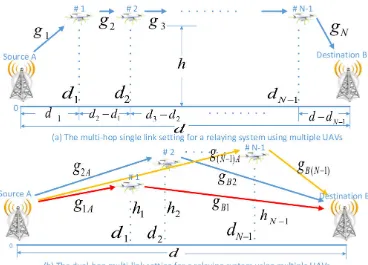
The relaying systems considered in this paper are shown in Fig. 1. In part (a), two ground
stations are used as source and destination nodes, and they are connected byN−1UAVs,N ≥3,
where the first UAV isd1 meters away from the source, the second UAV is d2 meters away from
the source and the last UAV is dN−1 meters away from the source. Thus, the distances between
the UAVs isdn−dn−1, wheren = 2,3,· · ·, N−1. The distance between the two ground stations
is d meters. All the UAVs have the same altitude of h meters. This gives the best performance.
The reason is that, if they have different altitudes, there will be a vertical distance between two
UAVs. In this case, according to the geometric theory, their distance becomes the square root
of the sum of the squared vertical distance and the squared horizontal distance. This will be
larger than their horizontal distance. Hence, the performance degrades due to a larger power
loss. Adaptive altitudes may only be useful when the propagation environments are different for
different UAVs, while this work assumes the same environment for all UAVs. In part (b), two
ground stations are still connected byN−1UAVs but instead of forming a multi-hop link, they
form N −1 relaying links assisted by the N −1 UAVs as independent dual-hop links. Each
UAV has an altitude of hn meters from the ground and a distance of dn meters away from the
source, n = 1,2,· · ·, N −1. In this case, the altitudes for different UAVs are different but their
optimal altitudes will be shown later to be the same, as this is determined by the propagation
environment. The total distance between the two ground stations is still d meters. Denote hmin
Figure 1. Diagrams for the multi-hop single link setting and the dual-hop multi-link setting of the
relaying system.
All UAVs adopt orthogonal channels by transmitting signals in different time slots but at the
same frequency band to avoid interference and to simplify the design. For the multi-hop setup,
N T seconds will be required to complete the whole transmission, whereT is the time duration of
the transmission in each hop andN is the number of hops. For the dual-hop setup, the source node
broadcasts the information in the first T seconds, and then each of theN−1UAVs forwards the
received information to the destination node in their designated time slots sequentially to avoid
interference at the destination. In this case, the total time required to complete the transmission
is still N T seconds. Thus, the two setups have the same total transmission time or latency.
Since they transmit signals over the same frequency band, they have the same spectral efficiency
as well. It is possible for different UAVs to be assigned different frequency bands to enable
simultaneous operations to reduce the latency, at the cost of a reduced spectral efficiency due to
increased bandwidth required.
settings. For example, the numbers of UAVs in each hop can be different, or different links may
have different hops. They can be considered as tradeoffs between distance and reliability. These
different relaying protocols offer flexibility, but they also lead to high networking overhead and
complicated control and synchronization due to dissimilar link settings. For aerial
communica-tions with remotely controlled moving nodes, this may not be preferable. Another issue related
to these protocols is the topology of the UAV relaying network. A detailed investigation of
different relaying protocols and their associated topologies can be an interesting future research
topic but is beyond the scope of the current work.
Note that the air channels in UAV communications are normally better than the
air-to-ground channels, as the path loss can be described by free-space propagation and is dominant
with less fading in the air-to-air channels, while fading may be dominant in the air-to-ground
channels due to objects near the ground stations, in addition to more severe path loss [28].
Nevertheless, all channels are assumed to have both path loss and fading. This leads to the
following observations. For the multi-hop single link setting, the communications distances are
shorter and most communications happen in the better air-to-air channels between different UAVs
with less power loss, but it does not have any diversity gain, as there is only a single link. On
the other hand, for the dual-hop multi-link setting, the communications distances are longer
and all communications happen in the worse air-to-ground channels between UAVs and ground
stations, but it has diversity gain due to the multiple relaying links. The diversity gain is the
rate at which the performance improves with signal-to-noise ratio, and it is proportional to the
number of independent links from the source to the destination in the relaying system [29].
Thus, it is interesting to know which setting offers the best overall performance. In order to do
this, the values of dn, hn and h need to be optimized so that one can compare the best possible
performances of both settings, which will be done in the next section. Next, we will discuss the
channel models.
Assume that the path loss for the air-to-air channel can be expressed as
LAA(r) =α110 log10r+η1, (1)
where α1 is the path loss exponent, r is the distance between two nodes and η1 is the path
loss at the reference point (1 meter in this case). This model applies to the channels between
equation, one will have α1 = 2 and η1 = 10 log10 4πfc 2
, where f is the carrier frequency and
c= 3×10⁸m/s is the speed of light.
Similarly, the path loss for the air-to-ground channel can be expressed as
LAG(r) = α210 log10r+η2, (2)
where α2, r and η2 are the path loss exponent, the distance and the path loss at the reference
point of the air-to-ground channel, respectively. This model applies to the channel between the
source node and the first UAV or the channel between the destination node and the last UAV.
The above equations are for the dB value of the path loss. For the absolute value, the air-to-air
and air-to-ground path loss models are
U(r) = 10LAA10(r) =β1rα1, (3)
and
V(r) = 10LAG10(r) =β2rα2, (4)
respectively, where β1 = 10η101 and β2 = 10
η2
10. For free-space propagation, η1 = 10 log
10 4πfc
2
so that β1 = 4πfc 2
.
A. Type A Channel Model
In this type, the path loss models have constant path loss exponent and reference path loss.
It has been revealed in many works that the air-to-air channel is very close to a free-space
propagation scenario. We use the results in [31] so that Type A channel model is given by
α1 = 2.05,
α2 = 2.32,
β1 =
4πf
c 2
,
β2 =
4πf
c 2
, (5)
where the air-to-ground channel has a larger path loss exponent than the air-to-air channel does.
A use case for this model is an aerial wireless sensor network, where several UAVs equipped
with sensors and radio devices fly over an area of interest to sense and collect data. More details
B. Type B Channel Model
In the second type, the to-air channel is determined by the Friis equation, while the
air-to-ground channel follows the model in [32] to give
α1 = 2,
α2 = 2,
β1 =
4πf
c 2
,
β2 = 10 B
10+
A
10+10a′e−b′(θ−a′), (6)
where A = ηLOS −ηN LOS, B = 10 log10 4πfc
2
+ηN LOS, θ = 180π arctan(dh1) is the angle of elevation, and a′, b′, η
LOS and ηN LOS depend on the propagation environment. For suburban
areas, a′ = 5.0188, b′ = 0.3511, η
LOS = 0.1dB and ηN LOS = 21dB. Note that the path loss
model here is also a function of the altitude h through the angle of elevation θ in β2 in (6).
Increasinghwill make the air-to-ground link closer to line of sight but at the same time increases
path loss [32]. Thus, the optimum altitude may exist. A use case for this model is a terrestrial
broadband radio access system, where the UAV acts as an aerial base station to provide coverage
for ground users in the system [32].
C. Type C Channel Model
In the third type, the air-to-air channel is still determined by free-space propagation, while
the air-to-ground channel follows the model in [33] such that
α1 = 2,
α2 = 3.9−0.9 log10h,
β1 =
4πf
c 2
,
β2 = 10−0.85h2.05, (7)
where h is the altitude. As reported in [33],1 ≤ h ≤ 120 meters in order for the model to be
valid. In this case, both the path loss exponent and the reference path loss in the air-to-ground
channel depend on the altitude but not on the distance. A use case for this model is the LTE
system, where the UAV acts as an aerial base station to serve the user equipment in the network,
D. End-to-End Performance
Using the above models, the end-to-end SNR of multi-hop AF relaying is shown as [30]
γee1 = " N
Y
i=1
(1 + 1
γi
)−1
#−1
, (8)
where γi is the SNR of the i-th hop with
γi =
Pi|gi|2
Wi·U(ri)
, i= 1or N,
γi =
Pi|gi|2
Wi·V(ri)
, i= 2,· · · , N −1, (9)
Pi is the transmission power of the i-th hop so that P1 is the transmission power of the source
node, P2 is the transmission power of UAV 1 and PN is the transmission power of UAV N−1,
gi is the fading coefficient of the i-th hop following Nakagami-m fading, Wi is the noise power
in the i-th hop so thatW1 is the noise power at UAV 1,WN−1 is the noise power at UAVN−1
and WN is the noise power at the destination node, andri is the distance of the i-th hop so that
r1 =ph2+d2
1, ri =di −di−1 for i= 2,· · · , N −1 and rN =
p
h2 + (d−d
N−1)2. Note that,
although both small-scale fading and large-scale path loss are considered in (9), in practice, the
direct use of (9) would lead to optimum positions that require knowledge of the instantaneous
channel state information and hence the optimum positions of the UAVs have to be adjusted
in real-time with energy-consuming acceleration and deceleration. A more practical solution is
to use the average SNR to optimize the UAV positions. This will give a suboptimal or rough
estimate of the optimum positions but can save energy for UAV operations.
We assume that gi follows a Nakagami m distribution with parameter m and average fading
power Ω and that all the fading coefficients are independent. Hence, we assume that both
air-to-air channels and air-to-ground channels suffer from path loss and fading. The Nakagami
m distribution is a very flexible fading model [35]. For example, when m = 1, it represents
Rayleigh fading, and when m→ ∞, it represents a non-fading channel. It can also approximate
the Rician fading with a one-to-one correspondence between m and the Rician K factor [35].
Although the Rician model is commonly used in UAV communications, it has been reported in
several works that the Nakagami model can be used to describe UAV channels too [36], [37].
For multi-hop DF relaying, the end-to-end SNR can be derived as
γee2 = min{γ1, γ2,· · · , γN}, (10)
The above is for the multi-hop setting. For the dual-hop multi-link setting, using selection
combining, the overall SNR of dual-hop AF that chooses the link with the largest end-to-end
link SNR is given by
χee1 = max
n {
γnAγBn
γnA+γBn+ 1}
, (11)
where n= 1,2,· · · , N −1 is the link index, γnAγBn
γnA+γBn+1 is the end-to-end SNR of the n-th link used for selection, γnA = PA|gnA|
2
Wn·V(rnA), γBn =
Pn|gBn|2
WB·V(rBn), PA is the transmission power of the source node, Pn is the transmission power of then-th UAV relay, gnA is the fading coefficient of
the channel between the source node and the n-th UAV relay, Wn is the noise power at the n-th
UAV, rnA =
p h2
n+d2n is the distance between the source node and the n-th UAV, gBn is the
fading coefficient of the channel between then−th UAV relay and the destination node, WB is
the noise power at the destination, and rBn=
p h2
n+ (d−dn)2 is the distance between the n-th
UAV and the destination. Also, gnA and gBn follow Nakagami m distributions with parameter
m and average fading power Ω. Thus, (11) is obtained by choosing the dual-hop link with the
largest link SNR from source to destination based on selection combining.
Note that selection combining is considered in this work due to its simplicity. There are other
combining schemes, such as maximum ratio combining or equal-gain combining. These schemes
often have better performances than selection combining but they require more channel
knowl-edge as well as incur more network overheads, which may not be desirable in the considered
applications, especially in relaying systems with more than one hop and more than two nodes.
Thus, they are not investigated here.
For multiple links using dual-hop DF, the end-to-end SNR is given by
χee2 = max
n {min{γnA, γBn}}. (12)
We will maximize the end-to-end SNR for different relaying protocols with respect to the
values of dn, hn and h in the next section.
III. PLACEMENTOPTIMIZATION
In order to compare the multi-hop single link setting with the dual-hop multi-link setting, we
need to find the optimum altitudes and distances that maximize the end-to-end SNR. We will do
this for three different types of channel models. Note that these models are suitable for different
A. Type A Channel Model
We start with the exact end-to-end SNR for multi-hop AF, γee1, as given in (8). From (8),
maximizingγee1 is equivalent to minimizingQNi=1(1 +γ1i). Thus, using (9), we need to minimize
the following value
Hee1(h, d1,· · ·, dN−1) = 1 +
W1β2(h2+d2 1)
α2
2
P1|g1|2
!
1 + WNβ2(h
2+ (d−d
N−1)2)
α2
2
PN|gN|2
!N−1 Y
i=2
1 + Wiβ1(di−di−1)
α1
Pi|gi|2
,h≥hmin, (13)
with respect to the altitude and the relevant distances. However, this optimization would give
optimum altitudes and distances as functions of the fading coefficients g1, g2,· · · , gN. Since
these fading coefficients are random, or at least change from time to time, the optimum altitudes
and distances have to change from time to time too. This may not be desirable in practice, as
acceleration and deceleration of the UAVs will consume a significant amount of energy. Also,
it may be difficult to obtain the channel state information. A simpler alternative is to first take
the average of (13) over the fading coefficients to eliminate the fading coefficients and then
optimize the average. Since the fading coefficients follow independent and identical Nakagami
m distributions with parameter m and average fading power Ω, the average of (13) can be
calculated as
Jee1(h, d1,· · · , dN−1) = 1 +
W1β2(h2+d2 1)
α2
2
P1Ω
!
1 + WNβ2(h
2+ (d−d
N−1)2)
α2
2
PNΩ
!N−1 Y
i=2
1 + Wiβ1(di−di−1)
α1
PiΩ
,h≥hmin, (14)
where several integrals of R∞ 0 (1 +
c x)(
m
Ω)m x
m−1
Γ(m)e−
m
Ωxdx are solved using [34, eq. (3.381.4)] to
give (1 + Ωc), c is a constant that equals to different values for different terms in (13) and
(m
Ω)
m xm−1
Γ(m)e
−m
Ωx is the probability density function of |gi|2 for i= 1,2,· · · , N. Hence, (14) can
simply be obtained from (13) by replacing the instantaneous fading power|gi|2 with the average
fading power Ω. Note that (14) is the average of (13), not the average end-to-end SNR. The
average end-to-end SNR is calculated by averaging (8) over the fading coefficients. However,
this calculation does not lead to any tractable expression for optimization, due to the inverse
function. Thus, it is not discussed here.
We use (14) as the target function for optimization in the following. For other channel models
by the averaging operation, the transmitters do not need the channel state information and will
not have this knowledge.
It can be shown that (14) is a convex function, as its second-order derivatives with respect
to h, d1,· · · , dN−1 are larger than 0. Similar arguments can also be made for other objective
functions, which are omitted in the paper. To optimize it by taking the first-order derivative of
(14) with respect to h, one has
∂Jee1 ∂h =
W1β2(h2+d21)
α2
2 −1α 2h
P1Ω
1 + W1β2(h2+d21)
α2
2
P1Ω
+
WNβ2(h2+(d−dN−1)2)
α2
2 −1α 2h
PNΩ
1 + WNβ2(h2+(d−dN−1)2)
α2
2
PNΩ
Jee1. (15)
One can see that (15) only equals to 0 when h = 0. Thus, in this case, the optimum altitude
would be ˆh= 0. In practice, since h≥hmin for safety reason, ˆh=hmin.
Also, by taking the first-order derivatives of (14) with respect to d1, d2,· · · , dN−1 and setting
them to zero, the optimum distances, d1,ˆ d2,ˆ · · · ,dˆN−1, satisfy
W1β2(ˆh2+ ˆd21)
α2
2 −1α 2dˆ1
P1Ω
1 + W1β2(ˆh2+ ˆd21)
α2
2
P1Ω
=
W2β1α1( ˆd2−dˆ1)α1−1
P2Ω
1 + W2β1( ˆd2−dˆ1)α1
P2Ω
=· · ·=
WNβ2(ˆh2+(d−dˆN−1)2)
α2
2 −1α
2(d−dˆN−1)
PNΩ
1 + WNβ2(ˆh2+(d−dˆN−1)2)
α2
2
PNΩ
. (16)
A special case occurs when the transmission SNRs at different nodes are the same. In this case, Pi
Wi = P
W for i= 1,2,· · · , N. Thus, from (16),
ˆ
d1 =d−dˆN−1 = ˆb,
ˆ
d2−d1ˆ = ˆd3−d2ˆ =· · ·= ˆdN−1−dˆN−2 = ˆa=
d−2ˆb
N −2, (17)
whereˆb is determined by
β2(ˆh2+ ˆb2)α2 2 −1α2ˆb
PΩ
W +β2(ˆh2+ ˆb2) α2
2
= β1α1(
d−2ˆb N−2)
α1−1
PΩ
W +β1( d−2ˆb N−2)α1
, (18)
for 0<ˆb < d2. One sees from (18) that, when the average SNR is large, the two denominators
are the same and can be cancelled out at both sides of the equation. In this case, the optimum
distances do not depend on the average SNR but only on the path loss model parameters, the
optimum altitude and the number of hops.
Next, we focus on the multi-hop DFγee2. Following exactly the same procedure, the objective
function to be minimized in this case is
Jee2(h, d1,· · · , dN−1) = max{
W1β2(h2+d2 1)
α2
2
P1Ω ,
W2β1(d2−d1)α1
P2Ω ,
· · · ,WNβ2(h
2+ (d−d
N−1)2)
α2
2
PNΩ }
Each element inside the maximum function is convex, as their second-order derivatives with
respect to h, d1,· · · , dN−1 are larger than 0. According to the convex optimization theory [38],
element-wise maximum preserves convexity so that the whole function in (19) is also convex.
Similar arguments can also be made for other objective functions, which are omitted in the paper.
The optimum altitude is again ˆh=hmin in practice. The optimum distances are derived from
W1β2(ˆh2+ ˆd2 1)
α2
2
P1Ω =
W2β1( ˆd2−d1ˆ)α1
P2Ω =· · ·=
WNβ2(ˆh2+ (d−dˆN−1)2)
α2
2
PNΩ
. (20)
In the special case when Pi Wi =
P
W, the optimum distances can be calculated from (17), where ˆb is determined by
β2(ˆh2+ ˆb2)α22 =β1(d−2ˆb
N −2)
α1. (21)
Next, we consider the dual-hop multi-link setting. In this case, the UAVs are independent so
that hn and dn can be optimized separately for different links. Thus, we can optimize the link
end-to-end SNR instead.
For χee1, it can be shown that one needs to minimize the objective function
Kee1(hn, dn) = 1 +
Wnβ2(h2n+d2n) α2
2
PAΩ
!
(1 + WBβ2(h
2
n+ (d−dn)2) α2
2
PnΩ
),hn≥hmin, (22)
for n= 1,2,· · · , N −1. By taking the first-order derivatives of (22) with respect tohn and dn,
it can be shown that the optimum altitude would be ˆhn = 0 but is hˆn =hmin in practice, and
the optimum distance is derived from
Wnβ2(ˆh2n+ ˆd2n) α2
2 −1α 2dˆn PAΩ
1 + Wnβ2(ˆh2n+ ˆd2n)
α2
2
PAΩ
=
WBβ2(ˆh2n+(d−dˆn)2) α2
2 −1α2(d−dˆn) PnΩ
1 + WBβ2(ˆh2n+(d−dˆn)2)
α2
2
PnΩ
. (23)
In the case when PA Wn =
Pn WB =
P
W, it can be easily derived that the optimum distance is dˆn = d
2.
Forχee2, the practical optimum altitude isˆhn =hmin and the optimum distance is determined
by
Wnβ2(ˆh2n+ ˆd2n) α2
2
PAΩ
= WBβ2(ˆh
2
n+ (d−dˆn)2) α2
2
PnΩ
. (24)
When PA
Wn = Pn WB =
P
W, the optimum distance is dˆn = d
2.
In summary, for the multi-hop single link setting, the practical optimum altitude is always
hmin, and the optimum distances can be obtained by solving N −1 nonlinear equations. When Pi
Wi = P
W, only one nonlinear equation needs to be solved. For the dual-hop multi-link setting, the practical optimum altitude is always hmin. The optimum distance can be found by solving
one nonlinear equation. In the case of PA Wn =
Pn
WB, the optimum distance is always d
B. Type B Channel Model
We start with the maximization of the exact end-to-end SNR for multi-hop AF as γee1. The
objective function is similar to that in (14), except that β2 is replaced by β2(h, d) to show its
dependence on h and d explicitly. The optimization method is also similar. Thus we only show
the final results to reduce the redundancy in the derivation. It can be shown that the optimum
altitude and distances satisfy
W1
P1Ω(ˆh
2+ ˆd2 1)
α2
2 [∂β2(ˆh,dˆ1)
∂ˆh +β2(ˆh,d1ˆ) α2hˆ
ˆ
h2+ ˆd2 1]
1 + W1β2(ˆh,dˆ1)(ˆh2+ ˆd21)
α2
2
P1Ω
+
WN PNΩ(ˆh
2+ (d−dˆ
N−1)2)
α2
2 [∂β2(ˆh,d−dˆN−1)
∂ˆh +β2(ˆh, d−dˆN−1)
α2ˆh
ˆ
h2+(d−dˆN
−1)2]
1 + WNβ2(ˆh,d−dˆN−1)(ˆh2+(d−dˆN−1)2)
α2
2
PNΩ
= 0, (25)
and
W1
P1Ω(ˆh
2+ ˆd2 1)
α2
2 [∂β2(ˆh,dˆ1)
∂dˆ1 +β2(ˆh,
ˆ
d1) α2dˆ1
ˆ
h2+ ˆd2 1]
1 + W1β2(ˆh,dˆ1)(ˆh2+ ˆd21)
α2
2
P1Ω
=
W2β1α1( ˆd2−dˆ1)α1−1
P2Ω
1 + W2β1( ˆd2−dˆ1)α1
P2Ω
=· · ·
=
WN PNΩ(ˆh
2+ (d−dˆ
N−1)2)
α2
2 [∂β2(ˆh,d−dˆN−1)
∂(d−dˆN−1) +β2(ˆh, d−
ˆ
dN−1) α2(d− ˆ
dN−1)
ˆ
h2+(d−dˆN
−1)2]
1 + WNβ2(ˆh,d−dˆN−1)(ˆh2+(d−dˆN−1)2)
α2
2
PNΩ
,
(26)
where one has from (6)
∂β2(h, x)
∂h =β2(h, x)
180xAln(10)
10π(h2+x2)
a′b′e−b′(180
π arctan(h/x)−a′)
(1 +a′e−b′(180
π arctan(h/x)−a′))2
,
∂β2(h, x)
∂x =−β2(h, x)
180hAln(10)
10π(h2+x2)
a′b′e−b′(180
π arctan(h/x)−a′)
(1 +a′e−b′(180
π arctan(h/x)−a′))2
. (27)
For multi-hop DF γee2, similarly, the optimum altitude and the optimum distances satisfy
∂β2(ˆh,d1ˆ)
∂ˆh +β2(ˆh,
ˆ
d1) α2ˆh
ˆ
h2+ ˆd2 1
= 0, (28)
and
W1
P1Ωβ2(ˆh,d1ˆ)(ˆh
2+ ˆd2 1)
α2
2 = W2β1( ˆd2−
ˆ
d1)α1
P2Ω =· · ·
= WN
PNΩ
β2(ˆh, d−dˆN−1)(ˆh2+ (d−dˆN−1)2)
α2
In the dual-hop multi-link setting, the procedures are very similar to before. In this case, for
dual-hop multi-link AFχee1, the optimum values of ˆhn anddˆn can be solved from the following
two nonlinear equations
Wn[∂β2(
ˆ
hn,dnˆ )
∂ˆhn +β2(ˆhn,dˆn) α2ˆhn
ˆ
h2n+ ˆd2n] PAΩ(ˆh2n+ ˆd2n)−
α2
2
1 + Wnβ2(ˆhn,dˆn)
PAΩ (ˆh
2
n+ ˆd2n) α2
2
+
WB[∂β2(
ˆ
hn,d−dnˆ )
∂ˆhn +β2(ˆhn,d−dˆn) α2ˆhn
ˆ
h2n+(d−dnˆ )2]
PAΩ(ˆh2n+(d−dˆn)2)− α2
2
1 + WBβ2(ˆhn,d−dˆn)
PAΩ (ˆh
2
n+ (d−dˆn)2) α2
2
= 0,
Wn[∂β2(
ˆ
hn,dnˆ )
∂dnˆ +β2(ˆhn,dˆn)
α2dnˆ ˆ
h2n+ ˆd2n] PAΩ(ˆh2n+ ˆd2n)−
α2
2
1 + Wnβ2(ˆhn,dˆn)
PAΩ (ˆh
2
n+ ˆd2n) α2
2
=
WB[
∂β2(ˆhn,d−dnˆ )
∂(d−dnˆ ) +β2(ˆhn,d−dˆn)
α2(d−dnˆ ) ˆ
h2n+(d−dnˆ )2]
PAΩ(ˆh2n+(d−dˆn)2)− α2
2
1 + WBβ2(ˆhn,d−dˆn)
PAΩ (ˆh
2
n+ (d−dˆn)2) α2
2
. (30)
For χee2, the two equations are
∂β2(ˆhn,dˆn)
∂ˆhn
+β2(ˆhn,dˆn)
α2ˆhn
ˆ
h2
n+ ˆd2n
= 0,
Wnβ2(ˆhn,dˆn)
(ˆh2
n+ ˆd2n)− α2
2 −
WBβ2(ˆhn, d−dˆn)
(ˆh2
n+ (d−dˆn)2)− α2
2
= 0. (31)
In summary, the optimum altitude and the optimum distances for the multi-hop single link
setting can be found by solving N nonlinear equations. In the special case when Pi Wi =
P W, it can be shown that one only needs to solve two nonlinear equations. For the dual-hop multi-link
setting, one needs to solve two nonlinear equations and in the special case, one nonlinear equation
for the optimum altitude and the optimum distance is always d2. In practice, the optimum altitude
takes the maximum of hmin and the solution from the equation.
C. Type C Channel Model
In this type, the path loss model parameters of the air-to-ground channel depend on the altitude
only. We use α2(h) and β2(h) to replace α2 and β2, respectively, to show this dependence
explicitly. They are defined in (7).
For the multi-hop AF, the optimum altitude satisfies
W1[∂β2(ˆh)
∂ˆh +β2(ˆh)( ∂α2(ˆh)
2∂ˆh ln(ˆh
2+ ˆd2 1) +
α2(ˆh)ˆh
ˆ
h2+ ˆd2 1)]
P1Ω(ˆh2+ ˆd2 1)
−α2(hˆ)
2 [1 + W1
P1Ωβ2(ˆh)(ˆh
2+ ˆd2 1)
α2(ˆh) 2 ]
+ WN[
∂β2(ˆh)
∂hˆ +β2(ˆh)( ∂α2(ˆh)
2∂ˆh ln(ˆh
2+ (d−dˆ
N−1)2) + hˆ2+(αd2−(ˆhdˆ)ˆNh
−1)2)]
PNΩ(ˆh2+ (d−dˆN−1)2)−
α2(hˆ)
2 [1 + WN
PNΩβ2(ˆh)(ˆh
2+ (d−d1ˆ)2)α2(2ˆh)]
and the optimum distances satisfy
W1β2(ˆh)
P1Ω (ˆh
2+ ˆd2 1)
α2(ˆh)
2 −1α2(ˆh) ˆd1
1 + W1β2(ˆh)
P1Ω (ˆh
2+ ˆd2 1)
α2(ˆh) 2
=
W2β1
P2Ω ( ˆd2−
ˆ
d1)α1−1α1
1 + W2β1
P2Ω ( ˆd2−
ˆ
d1)α1
=· · ·
=
WNβ2(ˆh)
PNΩ (ˆh
2+ (d−dˆ
N−1)2)
α2(hˆ)
2 −1α2(ˆh)(d−dˆN−1)
1 + WNβ2(ˆh)
PNΩ (ˆh
2 + (d−dˆ
N−1)2)
α2(ˆh) 2
, (33)
where
∂β2(h)
∂h = 2.05×10
−0.85h1.05,
∂α2(h)
∂h =−
0.9
hln 10. (34)
For multi-hop DF γee2, the optimum altitude and distances satisfy
∂β2(ˆh)
∂ˆh +β2(ˆh)(
∂α2(ˆh)
2∂ˆh ln(ˆh
2+ ˆd2 1) +
α2(ˆh)ˆh
ˆ
h2+ ˆd2 1
) = 0, (35)
W1β2(ˆh)
P1Ω (ˆh
2+ ˆd2 1)
α2(ˆh)
2 = W2β1
P2Ω ( ˆd2−d1ˆ)
α1 =· · ·= WNβ2(ˆh)
PNΩ
(ˆh2+ (d−dˆN−1)2)
α2(ˆh)
2 . (36)
Next, we discuss the dual-hop multi-link setting. In this case, for χee1, one has
Wn[∂β∂2ˆh(ˆhnn) +β2(ˆhn)(∂α2∂2(ˆˆhhnn)ln(ˆh2n+ ˆd2n) +
α2(ˆhn)ˆhn
ˆ
h2
n+ ˆd2n )]
PAΩ(ˆh2n+ ˆd2n)
−α2(ˆhn)
2 [1 + Wn
PAΩβ2(ˆhn)(ˆh
2
n+ ˆd2n) α2(hnˆ )
2 ]
+ WB[
∂β2(ˆhn)
∂ˆhn +β2(ˆhn)( ∂α2(ˆhn)
2∂hˆn ln(ˆh
2
n+ (d−dˆn)2) + hˆ2α2(ˆhn)ˆhn
n+(d−dˆn)2)]
PnΩ(ˆh2n+ (d−dˆn)2)− α2(hnˆ )
2 [1 + WB
PnΩβ2(ˆhn)(ˆh
2
n+ (d−dˆn)2) α2(ˆhn)
2 ]
= 0, (37)
Wnβ2(ˆhn) PAΩ (ˆh
2
n+ ˆd2n) α2(ˆhn)
2 −1dˆn
1 + Wnβ2(ˆhn)
PAΩ (ˆh
2
n+ ˆd2n) α2(ˆhn)
2
=
WBβ2(ˆhn) PnΩ (ˆh
2
n+ (d−dˆn)2) α2(ˆhn)
2 −1(d−dˆn)
1 + WBβ2(ˆhn)
PnΩ (ˆh
2
n+ (d−dˆn)2) α2(hnˆ )
2
, (38)
to find the optimum values of hn and dn. For χee2, one has
∂β2(ˆhn)
∂ˆhn
+β2(ˆhn)(
∂α2(ˆhn)
2∂ˆhn
ln(ˆh2n+ ˆd2n) + α2(ˆhn)ˆhn
ˆ
h2
n+ ˆd2n
) = 0, (39)
Wn
PAΩ
(ˆh2n+ ˆd2n)α2(2ˆhn) = WB
PnΩ
(ˆh2n+ (d−dˆn)2)
α2(ˆhn)
2 . (40)
In the above derivation, the results for the multi-hop AF and DF in three different UAV
channels have never been obtained in the literature before. The results for the dual-hop AF
special characteristics of Type B and Type C channels. The only result that is similar to those
in the literature [23] - [27] is the derivation for the dual-hop AF and DF in Type A channel.
Nevertheless, it is presented here for completeness and for comparison. Thus, most of our results
are new.
IV. PERFORMANCECOMPARISON
In this section, we compare the two relaying options using multiple UAVs in terms of the
outage and the bit error rate (BER). In [39], using the method proposed in [40], very accurate
approximations to the outage and the BER of multi-hop AF have been derived. In particular, for
γee1, one has the outage as [39]
PO(γth) =
1
2+
Z π2 0
Re{e
−jtanθ/γthΦ(tanθ)
jπtanθ }sec
2θdθ, (41)
whereRe{·}takes the real part of a complex number andΦ(·)is the characteristic function given
by Φ(ω) = M(s)|s=−jω, M(s) = QNi=1
2 Γ(m)
mˆcs
Γi
m2 Km(2
q
mˆcs
Γi )
is the moment-generating
function, Km(·) is them-th order modified Bessel function of the second type,cˆ=
PN
i=1Γ1i
QN
i=1(1+Γ1i)−1 is a constant, while Γi = WiPUiΩ(ri) for i = 1 or N and Γi = WiPViΩ(ri) for i = 2,· · · , N −1 is the
average SNR of the i-th hop. To find them, the optimum altitude and the optimum distances
derived in the previous section can be used to calculate ri.
Also, for γee1, the BER for binary phase shift keying is [39]
¯
Pe =
1
2 −
1
π Z π2
0
M(tanθ) sin(2√tanθ)
tanθ sec
2θdθ. (42)
For the multi-hop DF γee2, the outage and the BER can be calculated as [30]
PO(γth) = 1−
N
Y
i=1
(1− γ(m, mγth/Γi)
Γ(m) ), (43)
and
¯
Pe =
Z ∞
0 e−x
√ x[1−
N
Y
i=1
(1−γ(m, mx/Γi)
Γ(m) )]dx, (44)
respectively, where Γ(·) is the Gamma function and γ(·,·) is the incomplete Gamma function.
The outage probability of multi-hop DF is defined as PO(γth) = P r{γee2 < γth} in this
paper. Using (10), this gives P r{γee2 < γth} = P r{min{γ1, γ2,· · · , γN} < γth} = 1 −
P r{min{γ1, γ2,· · · , γN} > γth} = 1−QNi=1P r{γi > γth} = 1−QNi=1[1−P r{γi < γth}],
can be considered as the outage probability of the i-th hop. Thus, the overall outage of DF does
depend on the hop SNRs, either indirectly via the end-to-end SNR γee2 in P r{γee2 < γth} or
directly via the hop SNRs inP r{γi < γth}. These two methods are equivalent. Specifically, the
overall link will have an outage event as long as any of the hops have an outage event so that
the outage events in different hops are reflected in the overall outage.
For the dual-hop multi-link setting, since selection combining is used, one has the outage and
the BER as
PO =FN−1(γth), (45)
and
¯
Pe =
1 √
4π
Z ∞
0
FN−1(x)e −x
√
xdx, (46)
where one has [41]
F(x) = 1−2m
m(m−1)!e−Γ1mx−Γ2mx
Γm
2 Γ(m)Γ(m)
m1−1
X
i1=0
i1
X
i2=0
m−1 X
i3=0
i1
i2
m−1
i3
i1! (
m
Γ2
)i2−i23−1(m
Γ1
)2i1−i2+2 i3+1
x2i1+2m−2i2−i3−1(x+ 1)
i2+i3+1
2 Ki
2−i3−1(2
s
m2x(1 +x)
Γ1Γ2
), (47)
for AF χee1, and
F(x) = 1−(1− γ(m, mx/Γ1)
Γ(m) )(1−
γ(m, mx/Γ2)
Γ(m) ), (48)
for DF χee2. In the above equations, Γ1 = PΩ
W U(√h2
n+d2n)
and Γ2 = PΩ
W U(√h2
n+(d−dn)2)
, where hn
and dn can be replaced by the optimum altitude and distance calculated in the previous section.
These outage and BER expressions have been extensively studied and verified by simulation in
the literature. Interested readers can find more details in [39], [30] and [41] and the references
therein.
V. NUMERICALRESULTS AND DISCUSSION
In this section, numerical examples of the results derived in the previous sections are presented.
Since the optimum altitudes and distances depend on the average fading power only, no channel
fading is used to find these optimum locations but channel fading is used in the numerical results
to calculate the outage and bit error rate, as can be seen from Section IV. In the calculation,
we set P = 10 dBm, W = −100 dBm, m = 1 and Ω = 1. Other cases and settings can be
0 500 1000 1500 2000 2500 3000 3500 4000
d (m)
0 1000 2000 3000
Optimum a or b (m)
N=3
h=50 m
0 500 1000 1500 2000 2500 3000 3500 4000
d (m)
0 200 400 600 800
Optimum a or b (m)
N=7
[image:20.595.91.526.116.432.2]h=50 m
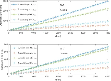
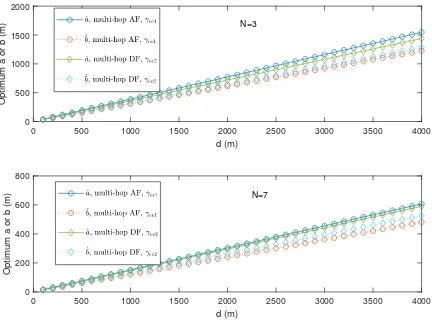
Figure 2. Optimum a and b vs. d for the multi-hop single link setting in Type A channel model.
A. Type A Channel Model
In this case, we set f = 2 GHz and the path loss model parameters are calculated by (5).
For Type A channel model, the optimum altitudes for both multi-hop single link and dual-hop
multi-link are zero or the minimum allowed safe altitude, and the optimum distance for the
dual-hop multi-link setting is always d2. Thus, they are not discussed here and we only examine the
optimum distances for the multi-hop single link setting. We set a practical limit ofhmin = 50m.
Note that the optimum distances can be calculated from the optimum a and b using (17).
Fig. 2 shows the optimumaandbvs. dfor the multi-hop single link setting in Type A channel
model. Several observations can be made. Firstly, the optimum values ofaandbincrease linearly
withd, whenN is fixed. This agrees with intuition, as the distances between nodes will increase
when they are used to cover a longer distance. Secondly, DF has a smaller ˆa than AF and
0 500 1000 1500 2000 2500 3000 3500 4000
d (m)
10-5 100
Outage
N=3
h=50 m
Multi-hop AF, ee1
Multi-hop DF,
ee2
Multi-link AF,
ee1
Multi-link DF,
ee2
0 500 1000 1500 2000 2500 3000 3500 4000
d (m)
10-6 10-4 10-2 100
BER
N=3
h=50 m
Multi-hop AF,
ee1
Multi-hop DF,
ee2
Multi-link AF,
ee1
[image:21.595.89.525.114.434.2]Multi-link DF, ee2
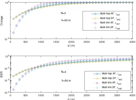
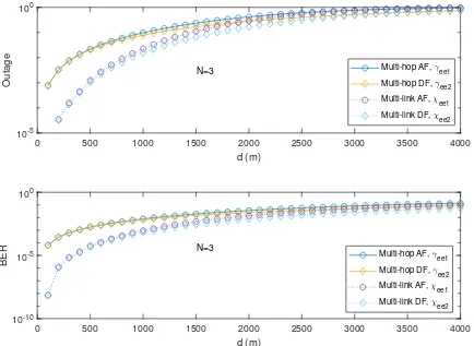
Figure 3. Outage and BER vs. d for Type A channel model when N = 3.
optimum UAV spacing is smaller and the distance between source (or destination) and the UAV
is larger than multi-hop AF. Thus, DF may be more suitable for a large disaster-affected area
that requires longer distance between the ground and the UAV. Thirdly, when N increases, the
spacing between nodes decreases, as expected. The difference between AF and DF also decreases
whenN increases. It can also be shown that the altitude has very limited effect on the optimum
values of a and b. To save space, it is not presented here.
Using the derived optimum distances, Figs. 3 and 4 compare the outage and BER performance
of the multi-hop single link setting with those of the dual-hop multi-link setting. Several important
observations can be made. Firstly, as the distance increases, the outage and BER performances
degrade in all cases, as more path loss will be incurred in each hop for a fixed number of UAV
relays. Secondly, the performance of the multi-hop single link setting is better than that of the
0 500 1000 1500 2000 2500 3000 3500 4000
d (m)
10-5 100
Outage
N=7
h=50 m
Multi-hop AF,
ee1
Multi-hop DF, ee2
Multi-link AF,
ee1
Multi-link DF, ee2
0 500 1000 1500 2000 2500 3000 3500 4000
d (m)
10-6 10-4 10-2 100
BER N=7
h=50 m
Multi-hop AF, ee1 Multi-hop DF,
ee2
Multi-link AF,
ee1
Multi-link DF,
[image:22.595.88.524.113.437.2]ee2
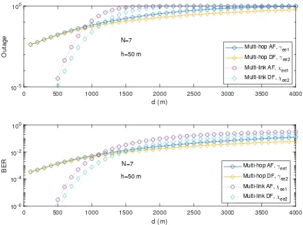
Figure 4. Outage and BER vs. d for Type A channel model when N = 7.
when N = 7, the multi-link setting has lower outage and BER than the multi-hop setting when
d < 1000 m. This important observation implies that, when multiple UAVs are used to cover
a long distance, one should form a multi-hop single link relaying system and otherwise form
a dual-hop multi-link relaying system. Our results quantify the threshold distances in different
cases for best design choices. Thirdly, it is also noted that DF outperforms AF in most cases for
both multi-hop and multi-link settings. Thus, DF is preferred in applications where performance
is more important than complexity.
B. Type B Channel Model
In this case, we consider the suburban area where a′ = 5.0188, b′ = 0.3511, η
LOS = 0.1dB
and ηN LOS = 21dB for (6). We choosef = 2GHz and hmin = 1 m. For the special case when
0 500 1000 1500 2000 2500 3000 3500 4000
d (m)
0 500 1000 1500 2000
Optimum a or b (m)
N=3
0 500 1000 1500 2000 2500 3000 3500 4000
d (m)
0 200 400 600 800
Optimum a or b (m)
[image:23.595.92.524.113.434.2]N=7
Figure 5. Optimum a and b vs. d in the multi-hop single link setting for Type B channel model.
multi-link setting are always d
2. Thus, we only examine the optimum distances for the multi-hop
single link setting and the optimum altitudes for both settings.
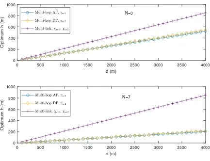
Fig. 5 shows the optimum a and b in the multi-hop single link setting. Again, the optimum
a and b increase linearly with d in the cases considered. The UAV spacing decreases when N
increases, and DF has a smaller optimum a and larger optimum b than AF. Fig. 6 shows the
optimumhin both settings, for Type B channel model. Since the optimum altitudes forχee1, and
χee2 are the same for the multi-link setting, there is only one curve for the multi-link case. One
can see that the optimum altitude in all cases increases linearly with the distance d. However,
the multi-link case has a larger optimum altitude than the multi-hop case, as high altitude is
required for the dual-hop multi-link setting in order to reduce path loss. The optimum altitude
for the multi-link case does not depend on N, as these UAVs operate independently for each
0 500 1000 1500 2000 2500 3000 3500 4000
d (m)
0 200 400 600 800 1000
Optimum h (m)
N=3
0 500 1000 1500 2000 2500 3000 3500 4000
d (m)
0 200 400 600 800 1000
Optimum h (m)
[image:24.595.90.523.110.442.2]N=7
Figure 6. Optimum h vs. d for Type B channel model.
means less spacing between UAVs and hence, lower altitude to keep the elevation angle.
Fig. 7 compares the multi-hop single link setting with the dual-hop multi-link setting. In this
case, there is no crossover between the multi-hop single link setting and the dual-hop multi-link
setting, but their performances are indistinguishable at large distances. In all cases, the
dual-hop multi-link setting outperforms the multi-dual-hop single link setting. Thus, for Type B channel
model, it is beneficial to use multiple UAVs to form a dual-hop multi-link relaying system. This
is because the diversity gain achieved by the multiple links always outweighs the smaller path
loss achieved by multiple hops, or the path loss in the air-to-ground channel is not large enough.
One can also see that DF is better than AF in this figure. Similar observations can be made for
0 500 1000 1500 2000 2500 3000 3500 4000
d (m)
10-5 100
Outage
N=3 Multi-hop AF, ee1
Multi-hop DF, ee2 Multi-link AF,
ee1
Multi-link DF,
ee2
0 500 1000 1500 2000 2500 3000 3500 4000
d (m)
10-10 10-5 100
BER
N=3
Multi-hop AF,
ee1
Multi-hop DF, ee2 Multi-link AF,
ee1
Multi-link DF,
[image:25.595.92.526.115.432.2]ee2
Figure 7. Outage and BER vs. d for Type B channel model when N = 3.
C. Type C Channel Model
In this model, we set f = 800 M Hz to be consistent with the measurement in [28]. Also,
the altitude is restricted as 1 ≤ h ≤ 120 m imposed by [28] so that hmin = 1 m. Since the
opitmum distance is always d2 for the dual-hop multi-link setting, we only examine the optimum
distances for the multi-hop single link setting and the optimum altitudes for both settings.
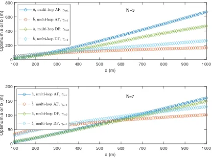
Fig. 8 shows the optimum a and b that can be used to calculate the optimum distances in
the multi-hop single link setting. In this figure, DF again has a smaller optimum a and a larger
optimum b than AF in most cases. Interestingly, unlike the other channel models, in Type C
channel model, ˆa crosses with ˆb, suggesting that for large distances of d, there should be less
spacing between source (or destination) and UAV than between UAVs. The threshold increases
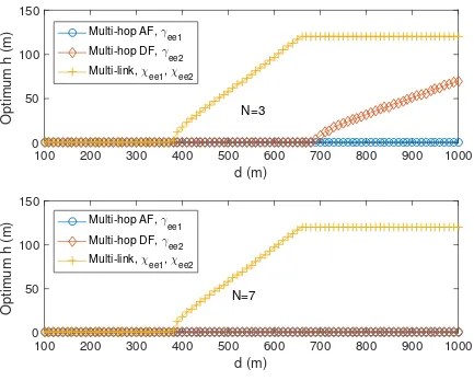
with N. Fig. 9 shows the optimum altitude for both settings in Type C channel model. There is
100 200 300 400 500 600 700 800 900 1000
d (m)
0 200 400 600 800
Optimum a or b (m)
N=3
100 200 300 400 500 600 700 800 900 1000
d (m)
0 50 100 150 200
Optimum a or b (m)
[image:26.595.92.525.114.439.2]N=7
Figure 8. Optimum a and b vs. d in the multi-hop single link setting for Type C channel model.
One can see that for multi-hop AF, the optimum altitude is always 1 meter in this figure, as in
these cases, the increase of path loss in β2 cannot be compensated by the decrease of the path
loss exponentα2, whenhincreases. For multi-hop DF, the observation is very similar, except that
whenN = 3, the optimum altitude starts to increase withdwhend >700m. On the other hand,
for the dual-hop multi-link setting, the optimum altitude starts from 1 meter and increases with
d when d > 400 m and then stay at 120 meters when d >650 m, suggesting that low altitude
should be used for small distance and high altitude should be used for large distance. This is
mainly caused by the limitation of the model in [28] that the altitude must be between 1 meter
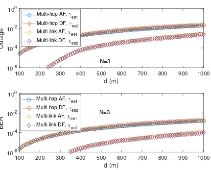
and 120 meters. Fig. 10 compares the multi-hop single link setting with the dual-hop multi-link
setting. In this case, the dual-hop multi-link setting always has smaller outage and BER than
the multi-hop single link setting, and the performance difference is considerable. Hence, the
100 200 300 400 500 600 700 800 900 1000
d (m)
0 50 100 150
Optimum h (m)
N=3Multi-hop AF, γ
ee1
Multi-hop DF, γ
ee2 Multi-link, χ
ee1, χee2
100 200 300 400 500 600 700 800 900 1000
d (m)
0 50 100 150
Optimum h (m)
N=7
Multi-hop AF, γ
ee1
Multi-hop DF, γ
ee2 Multi-link, χ
[image:27.595.91.524.111.459.2]ee1, χee2
Figure 9. Optimum h vs. d for Type C channel model.
Note that, in the most general case when all UAVs have different transmission SNRs, up toN
non-linear equations need to be solved in order to find the optimum altitudes and distances. The
computational complexity also increases whenN increases for larger systems. In our calculation,
we solved four non-linear equations in Type B channel model for 7 UAVs by using MATLAB
that runs on a desktop with i7-3770 CPU and 16 G memory. This takes about 2.4 seconds,
which seems to be reasonable. Also, N cannot be too large, as this not only increases the
computational complexity but also increases the control overhead too. It is very difficult to
implement coordination and collision avoidance for a large swarm. Thus, practical systems may
not have a large N. Moreover, the computation is on-off and can be performed offline, as the
parameters of d, Ω, P and W are normally fixed. Thus, even for large systems, as long as the
computation is performed well in advance, this may not be an issue. Finally, if the UAVs use
100 200 300 400 500 600 700 800 900 1000
d (m)
10-6 10-4 10-2 100
Outage
N=3
Multi-hop AF, γ
ee1
Multi-hop DF, γ
ee2 Multi-link AF, χ
ee1 Multi-link DF, χ
ee2
100 200 300 400 500 600 700 800 900 1000
d (m)
10-6 10-4 10-2 100
BER
N=3
Multi-hop AF, γ
ee1
Multi-hop DF, γ
ee2 Multi-link AF, χ
ee1 Multi-link DF, χ
[image:28.595.94.525.105.452.2]ee2
Figure 10. Outage and BER vs. d for Type C channel model when N = 3.
need to be solved so that the complexity does not scale up with N. Note also that the results
are presented here in terms of outage and bit error rate, while the optimization is performed for
the SNR. It is very difficult to optimize the outage and the bit error rate with respect to the
placement directly, due to the non-linear relationship between the SNR and the outage or bit
error rate. In fact, as can be seen from Section IV, the outage and bit error rate do not have any
closed-form expressions for optimization in most cases. Thus, we maximize the SNR instead,
as a higher SNR generally leads to better outage and bit error rate performances.
VI. CONCLUSION
In this paper, the use of multiple UAVs in wireless relaying has been studied. The optimum
positions of the UAVs in two typical relaying options of a single multi-hop link and multiple
AF and DF. The outage and the BER performances of these two options have been compared.
Numerical results have shown that the multiple dual-hop links option is preferred in
air-to-ground channels whose path loss parameters are functions of UAV positions. When the path
loss parameters are independent of UAV positions, the multi-hop single link is a better option
only for large distances between source and destination. In the comparison, it has also been
shown that DF is a better option than AF. These optimizations require solutions to complicated
non-linear equations. However, this only needs to be done once and can be performed offline
by the ground controller before the launch of the UAV, as the optimum positions depend on
constants in the propagation environment that do not change with time.
REFERENCES
[1] S. Hayat, E. Yanmaz, and R. Muzaffar, ”Survey on unmanned aerial vehicle networks for civil applications: a
communications viewpoint,” IEEE Commun. Surveys and Tutorials, vol. 18, pp. 2624-2661, 4th Quarter 2016.
[2] Y. Zeng, R. Zhang, and T.J. Lim, ”Wireless communications with unmanned aerial vehicles: opportunities and challenges,”
IEEE Comm. Mag., vol. 54, pp. 36 - 42, May 2016.
[3] A. Jaziri, R. Nasri, and T. Chahed, ”Congestion mitigation in 5G networks using drone relays,”Proc. IEEE WCNC 2016,
pp. 233 - 238, 2016.
[4] A. Osseiran, F. Boccardi, V. Braun , ”Scenarios for 5G mobile and wireless communications: the vision of the METIS
project,”IEEE Commun. Mag., vol. 52, pp. 26 - 35, May 2014.
[5] R. Lee, J. A. Manner, J. Kim, P. Amodio, and K. Anderson, ”White Paper: The Role of deployable aerial communications
architecture in emergency communications and recommended next steps,” FCC Public Safety and Homeland Security
Bureau, Sept. 2011.
[6] D. Orfanus, E.P. de Freitas, F. Eliassen, ”Self-organization as a supporting paradigm for military UAV relay networks,”
IEEE Commun. Lett., vol. 20, pp. 804 - 807, 2016.
[7] Y. Chen, W. Feng, G. Zheng, ”Optimum placement of UAV as relays,” accepted byIEEE Communications Letters.
[8] M. Mozaffari, W. Saad, M. Bennis, M. Debbah, ”Unmanned aerial vehicle with underlaid device-to-device communications:
performance and tradeoffs,”IEEE Trans. Wireless Commun., vol. 15, pp. 3949 - 3963, June 2016.
[9] M. Mozaffari, W. Saad, M. Bennis, M. Debbah, ”Optimal transport theory for cell association in UAV-enabled cellular
networks,”IEEE Commun. Lett., vol. 21, pp. 2053 - 2056, Sept. 2017.
[10] N. Zhao, F.R. Yu, Y. Chen, G. Gui, ”Caching UAV assisted secure transmission in hyper-dense networks based on
interference alignment,” accepted byIEEE Trans. Communications.
[11] F. Cheng, S. Zhang, Z. Li, Y. Chen, N. Zhao, R. Yu, V.C.M. Leung, ”UAV trajectory optimization for data offloading at
the edge of multiple cells,” accepted byIEEE Transactions on Vehicular Technology.
[12] Y. Zeng, R. Zhang, and T.J. Lim, ”Throughput maximization for UAV-enabled mobile relaying systems,” IEEE Trans.
Commun., vol. 64, pp. 4983 - 4996, Dec. 2016.
[13] Q. Wang, Z. Chen, W. Mei, and J. Fang, ”Improving physical layer security using UAV-enabled mobile relaying,”IEEE
Wireless Commun. Lett., vol. 6, pp. 310 - 313, June 2017.
[14] F. Ono, H. Ochiai, and R. Miura, ”A wireless relay network based on unmanned aircraft system with rate optimization,”
[15] I.Y. Abualhaol, M.M. Matalgah, ”Performance analysis of multi-carrier relay-based UAV network over fading channels,”
Proc. IEEE Globecom 2010 Workshop on Wireless Networking for Unmanned Aerial Vehicles, pp. 1811 - 1815, 2010.
[16] P. Zhan, K. Yu, A.L. Swindlehurst, ”Wireless relay communications using an unmanned aerial vehicle,” IEEE SPAWC
2006, pp. 1 - 5, 2006.
[17] E. Larsen, L. Landmark, and Ø. Kure, ”Optimal UAV relay positions in multi-rate networks,”IEEE Wireless Days, pp. 8
- 14, 2017.
[18] I. Rubin and R. Zhang, ”Placement of UAVs as communication relays aiding mobile ad hoc wireless networks,” Proc.
IEEE Military Communications Conference 2007, pp. 1 - 7, 2007.
[19] P. Ladosz, H. Oh, and W.-H. Chen, ”Optimal positioning of communication relay unmanned aerial vehicles in urban
environments,”Proc. 2016 International Conference on Unmanned Aircraft Systems (ICUAS), Arlington, USA, June 2016.
[20] M. Horiuchi, H. Nishiyama, N. Kato, F. Ono, and R. Miura, ”Throughput maximization for long-distance real-time data
transmission over multiple UAVs,”2016 IEEE International Conference on Communications, pp. 1 - 6, 2016.
[21] P. Vincent, I. Rubin, ”A framework and analysis for cooperative search using UAV swarms,”ACM Symposium on Applied
Computing. pp. 79 - 86, 2004.
[22] H. Shakhatreh, A. Khreishah, J. Chakareski, ”On the continuous coverage problem for a swarm of UAVs,” 2016 IEEE
Sarnoff Symposium, 2017.
[23] J. Cannons, L.B. Milstein, K. Zeger, ”An algorithm for wireless relay placement,”IEEE Trans. Wireless Commun., vol. 8,
pp. 5564 - 5574, Nov. 2009.
[24] A. Ribeiro, X. Cai, G. Giannakis, ”Symbol error probabilities for general cooperative links,”IEEE Trans. Wireless Commun.,
vol. 4, pp. 1264 - 1273, May 2005.
[25] A. Nasri, R. Schober, I.F. Blake, ”Performance and optimization of amplify-and-forward cooperative diversity systems in
generic noise and interference,”IEEE Trans. Wireless Commun., vol. 10, pp. 1132 - 1143, Apr. 2011.
[26] B. Zhu, J. Cheng, M.-S. Alouini, L. Wu, ”Relay placement for FSO multihop DF systems with link obstacles and infeasible
regions,”IEEE Trans. Wireless Commun., vol. 14, pp. 5240 - 5250, Sept. 2015.
[27] M. Bagaa, A. Chelli, D. Djenouri, T. Taleb, I. Balasingham, K. Kansanen, ”Optimal placement of relay nodes over limited
positions in wireless sensor networks,”IEEE Trans. Wireless Commun., vol. 16, pp. 2205 - 2219, Apr. 2017.
[28] N. Goddemeier and C. Wietfeld, ”Investigation of air-to-air channel characteristics and a UAV specific extension to the
Rice model,”2015 IEEE Globecom, pp. 1 - 5, 2015.
[29] Y. Jing and H. Jafarkhani, ”Single and multiple relay selection schemes and their achievable diversity orders,”IEEE Trans.
Wireless Commun., vol. 8, pp. 1414 - 1423, Mar. 2009.
[30] M.O. Hasna and M.-S. Alouini, ”Outage probability of multihop transmission over Nakagami fading channels,” IEEE
Commun. Lett., vol. 7, pp. 216 - 218, May 2003.
[31] N. Ahmed, S.S. Kanhere, and S. Jha, ”On the importance of link characterization for aerial wireless sensor networks,”
IEEE Commun. Mag., vol. 54, pp. 52 - 57, May 2016.
[32] A. Al-Hourani, S. Kandeepan, S. Lardner, ”Optimal LAP altitude for maximum coverage,”IEEE Wireless Commun. Lett.,
vol. 3, pp. 569 - 572, Dec. 2014
[33] R. Amorim, H. Nguyen, P. Mogensen, I.Z. Kov´acs, J. Wigard, T.B. Sørensen, ”Radio channel modelling for UAV
communication over cellular networks,”IEEE Wireless Commun. Lett., vol. PP, pp. 1-1, 2017.
[34] I.S. Gradshteyn, I.M. Ryzhik,Table of Integrals, Series, and Products, 6th Ed. San Diego, CA: Academic Press. 2000.
[35] M.K. Simon and M.-S. Alouini,Digital Communication Over Fading Channels, 2nd Ed. John Wiley& Sons: London, 2000.
[36] W. Khawaja, I. Guvenc, and D. Matolak, ”UWB channel sounding and modeling for UAV air-to-ground propagation
[37] E. Yanmaz, R. Kuschnig, and C. Bettstetter, ”Achieving air–ground communications in 802.11 networks with
three-dimensional aerial mobility,” inProc. IEEE INFOCOM, Turin, Italy, April 2013, pp. 120-124.
[38] S. Boyd,Convex Optimization, Cambridge University Press: Cambridge, UK. 2004.
[39] N.C. Beaulieu, G. Farhadi, and Y. Chen, ”A precise approximation for performance evaluation of amplify-and-forward
multihop relaying systems,”IEEE Trans. Wireless Commun., vol. 10, pp. 3985 - 3989, Dec. 2011.
[40] N.C. Beaulieu, Y. Chen, ”An accurate approximation to the average error probability of cooperative diversity in Nakagami-m
fading,”IEEE Trans. Wireless Commun., vol. 9, pp. 2707 - 2711, Sept. 2010.
[41] A. Bletsas, H. Shin, and M. Z. Win, ”Outage optimality of opportunistic amplify-and-forward relaying,”IEEE Commun.