warwick.ac.uk/lib-publications
Original citation:Branke, Juergen, Corrente, Salvatore, Greco, Salvatore and Gutjahr, Walter. (2017) Efficient pairwise preference elicitation allowing for indifference. Computers & Operations Research, 88 . pp. 175-186.
Permanent WRAP URL:
http://wrap.warwick.ac.uk/89589
Copyright and reuse:
The Warwick Research Archive Portal (WRAP) makes this work by researchers of the University of Warwick available open access under the following conditions. Copyright © and all moral rights to the version of the paper presented here belong to the individual author(s) and/or other copyright owners. To the extent reasonable and practicable the material made available in WRAP has been checked for eligibility before being made available.
Copies of full items can be used for personal research or study, educational, or not-for-profit purposes without prior permission or charge. Provided that the authors, title and full bibliographic details are credited, a hyperlink and/or URL is given for the original metadata page and the content is not changed in any way.
Publisher’s statement:
© 2017, Elsevier. Licensed under the Creative Commons Attribution-NonCommercial-NoDerivatives 4.0 International http://creativecommons.org/licenses/by-nc-nd/4.0/
A note on versions:
The version presented here may differ from the published version or, version of record, if you wish to cite this item you are advised to consult the publisher’s version. Please see the ‘permanent WRAP url’ above for details on accessing the published version and note that access may require a subscription.
Efficient Pairwise Preference Elicitation
Allowing for Indifference
Juergen Brankea, Salvatore Correnteb, Salvatore Grecob,c, Walter Gutjahrd aWarwick Business School, The University of Warwick, Coventry, CV4 7AL, United
Kingdom
bDepartment of Economics and Business, University of Catania, Corso Italia, 55, 95129 Catania, Italy
cOperations and Systems Management, Portsmouth Business School, Portsmouth PO1 3DE, United Kingdom
dUniversity of Vienna, 1090 Wien, Austria
Abstract
Many methods in Multi-Criteria Decision Analysis for choice problems rely on eliciting pairwise preference information in their attempt to efficiently identify the most preferred solution out of a larger set of solutions. That is, they repeatedly ask the decision maker which of two solutions is preferred, and then use this information to reduce the number of possibly preferred solutions until only one remains. However, if the solutions have a very similar value to the decision maker, he/she may not be able to accurately decide which solution is preferred. This paper makes two main contributions. First, it extends Robust Ordinal Regression to allow a user to declare indifference in case the values of the two solutions do not differ by more than some personal threshold. Second, we propose and compare several heuristics to pick pairs of solutions to be shown to the decision maker in order to minimize the number of interactions necessary.
Keywords: Multi-Criteria Decision Analysis, pairwise preference elicitation, indifference, efficient information collection, robust ordinal regression
1. Introduction
alternatives and criteria. Multi-Criteria Decision Analysis (MCDA) supports users in this task, and a variety of methods have been proposed. Robust Ordinal Regression (ROR) [24] elicits pairwise preference information from the DM, and uses this information together with an assumed underlying preference model to derive additional preference relations and thereby enrich the preference ordering. A key advantage of ROR is that it simultaneously takes into account all value functions compatible with the DM’s preference information.
In practice, it may be difficult for a DM to specify which of two solutions is more preferred if these solutions have a very similar value (note that they may be quite different, but have different strengths and weaknesses so that overall, they constitute a similar value to the DM). In such cases, forcing a DM to make a choice is likely to lead to errors, which can then lead to inconsistencies in the preference information such as intransitivity of preferences (the user may state that a is preferred over b, b is preferred over c, but c is preferred overa). This, in turn, may lead to an empty set of compatible value functions and abortion of the method. A few papers have proposed mechanisms to deal with inconsistent preference information, and usually suggest to discard the oldest preference information (e.g., [35]).
In our paper, we extend ROR to allow the DM to declare indifference between two solutions in case the values of the two solutions are similar. In particular, we assume that the DM has a personal internal (unknown to our method) “precision threshold” δT, and will declare indifference if the
differ-ence in value between the two solutions is withinδT, i.e.,|U(a)−U(b)| ≤ δT, where U(a) denotes the utility or value of alternative a. This means that we are supposing that the preference relation% over the set of considered alter-natives is a semiorder, that is, %is strongly complete, Ferrers transitive and semitransitive (see [16]). Our extended version of ROR will attempt to learn the DM’s precision threshold along with their value function. This approach is easier on the DM and avoids the complications of forcing the DM to specify a preference even if the alternatives have very similar values.
Let us underline that the meaning of the threshold δT used in the paper is
between two alternatives [33].
We propose two basic algorithms for this scenario, one that attempts to identify all solutions acceptable to the DM (note that because of the DM’s indifference threshold, it may happen that there are several solutions that are equally acceptable to the DM), and one that attempts to identify at least one acceptable solution.
Furthermore, in this paper we propose several heuristics to pick the pairs of solutions to be shown to the DM with the goal to minimize the expected number of interactions necessary to identify the most preferred solution. To test ROR with indifference information and these heuristics, we propose a configurable benchmark generator that allows to generate a wide range of artificial benchmark problems.
The paper is structured as follows. We start in Section 2 with an overview on related work. Section 3 defines some fundamental concepts when allowing for indifference information. The actual algorithms implementing a version of ROR that allows for indifference information can be found in Section 4. The heuristics to speed up convergence are explained in Section 5, followed by empirical evaluation in Section 6. The paper concludes with a summary and some ideas for future work in Section 7.
2. Related work
2.1. Multi-Criteria Decision Analysis and value functions
MCDA (see [15, 23]) is a methodology to support complex decisions in which a plurality of criteria have to be taken into consideration. In the MCDA perspective, the basic elements of a decision problem are the set of alternatives A={a, b, ...}, that can be either finite or infinite (in this paper we consider finite set A, only), and the set of criteria G = {g1, . . . , gm} by
which the alternatives from Aare evaluated [38]. Without loss of generality, each criterion gj ∈ G can be considered as a real-valued function gj : A →
Ij ⊆R, such that for all a, b∈A,gj(a)≥gj(b) if and only ifa is at least as
good as b on criteriongj and Ij ={gj(a) :a∈A}1. In the following, for the
sake of simplicity, sometimes we identify the criteria gj with their indices j.
MCDA deals with the following three basic decision problems [39]:
1Therefore,I
• the choice problem, in case the best alternative or a small set composed of the best alternatives have to be selected;
• the sorting problem, in case each alternative has to be assigned to some pre-defined and ordered categories;
• the ranking problem, in case the alternatives have to be ordered from the best to the worst.
In this paper we shall consider only the choice problem. When for a and b from A, gj(a)≥ gj(b) for all criteria gj ∈ G one says that a (weakly)
domi-nates b, and in this case, there is no doubt that ais comprehensively at least as good as b. However, in practical problems, dominance is rarely observed and, therefore, to compare at a comprehensive level alternatives fromA it is necessary to aggregate the evaluations assigned to the alternatives by criteria from G. Very often a value function representing the overall desirability of alternatives a ∈ A by means of a synthesis of their evaluations on criteria gj ∈G is considered. Formally a value function U :
Qm
j=1Ij → R, assigns a
value to each alternative from A such that for any a, b ∈ A, a is at least as good as b (a % b) if and only if U(g1(a), . . . , gm(a))≥U(g1(b), . . . , gm(b)).
Very often the value function U is assumed to be additive [30, 49], that is, for all a∈A
U(g1(a), . . . , gm(a)) = m
X
j=1
uj(gj(a)), (1)
with uj(gj(a)) non-decreasing for all gj ∈G.
A special case of the additive form of the value function U, very widely used in the literature and in the applications, is the weighted sum, that is
U(g1(a), . . . , gm(a)) = m
X
j=1
wjgj(a), (2)
with wj ≥0 for all gj ∈G and
Pm
j=1wj = 1.
acceleration have surely a relevant weight. However, in general cars with a high maximum speed have also a good acceleration and there is therefore the risk of an over-evaluation of those cars. Thus, we can say that there is redundancy between the criteria of maximum speed and acceleration. This can be explained by saying that the weight of the two criteria maximum speed and acceleration considered together is smaller than the sum of the weight of the two criteria considered separately. On the other hand, still for a DM interested in sports cars, price is not a criterion as relevant as maximum speed. However, since in general a car with a good maximum speed is expensive, a car having both a good maximum speed and a good price is particularly appreciated. Thus we can say that there is synergy between the criteria of maximum speed and price. This can be explained by saying that the weight of the two criteria maximum speed and price considered together is greater than the sum of the weight of the two criteria considered separately. To model redundancy and synergy between criteria a widely used model is the Choquet integral [10]. It is based on a representation of weight of criteria in terms of a capacity, which assigns to each subset of criteria T ⊆ G, the valueµ(T) corresponding to the total weight of criteria from T. The weights µ(T), T ⊆ G, are not required to be additive, which means that for any S, R ⊆ G such that S ∩R = ∅, one can have µ(S ∪T) = µ(S) +µ(T) in case there is neither redundancy nor synergy between S and T, but also µ(S∪T)< µ(S) +µ(T) in case of redundancy, andµ(S∪T)> µ(S) +µ(T) in case of synergy. Formally, denoting by 2G the power set of G being the
set of all subsets of G, the capacity µ is a set function µ : 2G → [0,1] that satisfies the following properties:
1a) µ(∅) = 0 and µ(G) = 1 (boundary conditions),
2a) ∀S ⊆T ⊆G, µ(S)≤µ(T) (monotonicity condition).
Givena∈A and a capacityµon 2G, the Choquet integral (for application of
Choquet integral to MCDA see [21]), as above explained, gives the analogous of the weighted sum in case of additive weights, and it is defined as follows:
Cµ(a) = m
X
i=1
g(i)(a)−g(i−1)(a)
µ {gj ∈G:gj(a)≥g(i)(a)}
whereg(·)reorders the criteria so thatg(1)(a)≤. . .≤g(m)(a), andg(0)(a) = 0.
A useful concept dealing with the Choquet integral is the M¨obius represen-tation of the capacity µ being the function m : 2G → R [37, 43] such that, for all S ⊆G
µ(S) = X
T⊆S
m(T). (4)
Equation (4) is equivalent to
m(S) = X
T⊆S
(−1)|S−T|µ(T) (5)
which permits to easily compute the M¨obius representation.
The properties 1a) and 2a) can be reformulated also in terms of the M¨obius representation [9] as follows:
1b) m(∅) = 0, X
T⊆G
m(T) = 1,
2b) ∀i∈G and ∀R⊆G\ {i}, m({i}) + X
T⊆R
m(T ∪ {i})≥0.
The M¨obius representation permits to express the Choquet integral in a linear form as a weighted sum of minimum values given to the considered alternative a∈A by all subsets of criteria T fromG [20],
Cµ(a) =
X
T⊆G
m(T) min
i∈T gi(a). (6)
Observe that the terms m(T) min
i∈T gi(a) in (6) can be interpreted as
repre-senting the contribution of the interaction between criteria from T ⊆ G to the overall evaluation Cµ(a) of alternative a ∈A. In order to handle a
sim-pler decision model, in many applications it seems reasonable to take into account interactions between no more than k criteria. This is obtained by putting m(T) = 0 if |T| > k and the corresponding capacities are called k-additive [22]. Very frequently 2-additive capacities are used so that the M¨obius representation and the corresponding Choquet integral become
µ(S) =X
i∈S
m({i}) + X {i,j}⊆S
Cµ(a) =
X
i∈G
m({i})gi(a) +
X
{i,j}⊆G
m({i, j})min{gi(a), gj(a)}. (8)
Moreover, properties 1b) and 2b) reduce to
1c) m(∅) = 0, X
i∈G
m({i}) + X {i,j}⊆G
m({i, j}) = 1,
2c)
m({i})≥0, ∀i∈G,
m({i}) +X
j∈T
m({i, j})≥0, ∀i∈Gand∀T ⊆G\ {i}, T 6=∅.
2.2. Ordinal Regression and Robust Ordinal Regression
Each decision model requires specification of some parameters. For ex-ample, if one adopts the additive value function (1), it is necessary to define the parameters related to the formulation of the marginal value functions uj(gj(a)), j = 1, . . . , m. Eliciting directly the parameters of the adopted
de-cision model from the DM in real-world dede-cision making situations requires a technical background from the DM that in general is not reasonable to expect. Moreover, even in the case that the DM has such a background, a high cognitive effort is required so that, in any case, the preference informa-tion elicited in this way is not reliable enough. Consequently, within MCDA, many methods have been proposed to determine the parameters characteriz-ing the considered decision model in an indirect way, i.e., induccharacteriz-ing the values of parameters in the adopted decision model, from some holistic preference comparisons of alternatives given by the DM. This indirect preference elici-tation does not require any technical background and requires a quite mild cognitive effort. The use of such an indirect preference information is the basis of the ordinal regression paradigm.
The ordinal regression methodology (for a survey see [44]) was proposed by Jacquet-Lagr`eze and Siskos [27] that introduced the UTA (UTilit´es Addi-tives) method which aims at inferring one or more additive value functions in the form (1) from some preference information expressed by the DM in terms of pairwise comparisons of some from alternatives A, so that, for a, b∈A:
• a DM b if for the DM alternative a is preferred to alternative b (that is
a%DM b and not(b%DM a)),
• a∼DM b if for the DM alternative a is indifferent to alternative b (that is
a%DM b and b%DM a).
Technically, ordinal regression requires to solve an optimization problem of the type:
max ε, s.t.
U(a)≥U(b) if a%DM b, with a, b∈A,
U(a)≥U(b) +ε if aDM b, witha, b∈A,
U(a) = U(b) if a∼DM b, witha, b∈A,
EHP C
constraints related to the analytical form of the adopted value function
EAF
EOR (9)
The nature of the optimization problem (9) depends on the form of the value function. Generally it is a linear programming problem. This is the case of additive value functions (1), weighted sum value functions (2) and of the value function in the form of the Choquet integral (3).
If the set of constraintsEORis feasible andε∗ >0, withε∗ = max ε, then there exists at least one value function of the considered form that is compat-ible with the preference information supplied by the DM. On the contrary, if there is no compatible value function, one can select the value function U on the considered class that minimizes the sum of deviation errors or the number of ranking errors in the sense of Kendall or Spearman distance [27]. When there is a compatible value function, in general, there is a plurality of value functions of the selected class (e.g. weighted sum, additive value func-tion, Choquet integral) that permits to represent the preference information supplied by the DM. The methods proposed within the ordinal regression paradigm select one of these value functions according to some predefined principle. One has to admit that to take into consideration only one of the many compatible value functions is always arbitrary to some extent. Because of this observation, Greco et al. [24] proposed to take into account the whole setU of value functions compatible with the preference information supplied by the DM through a methodology called Robust Ordinal Regression (for some surveys see [12, 13, 25]) that is based on the necessary and possible preference relations %N and
%P defined as follows:
• a%P b iff U(a)≥U(b) for at least one U ∈ U, witha, b∈A.
Necessary and possible preferences%N and%P onAare characterized by the following properties [19]:
• %N is a partial preorder onA,
• %N⊆
%P,
• a%N b and b%P c ⇒ a%P c, ∀a, b, c∈A,
• a%P b and b %N c ⇒ a%P c, ∀a, b, c∈A,
• a%N b orb%P a, ∀a, b∈A.
To compute the necessary and possible preference relations one has to con-sider the following sets of constraints,
U(b)≥U(a) +ε EOR,
EN(a, b) U(a)≥U(b) EOR.
EP(a, b)
We have that:
• a %N b if EN(a, b) is infeasible or if εN ≤0 where εN = maxε subject to EN(a, b),
• a %P b if EP(a, b) is feasible and εP > 0 where εP = maxε subject to
EP(a, b).
the DM based on the Hit-And-Run procedure (HAR; [45, 46]). For an ex-tension of this SMAA methodology to the case of value functions expressed as Choquet integral see [3].
In case of a value function expressed as a Choquet integral with respect to a 2-additive capacity, the linear programming problem related to ordinal regression becomes [34]:
max ε, s.t.
Cµ(a)≥Cµ(b) ifa%DM b,
Cµ(a)≥Cµ(b) +εifaDM b,
Cµ(a) = Cµ(b) ifa∼DM b,
EHP C
m({∅}) = 0, P
i∈G
m({i}) + P {i,j}⊆G
m({i, j}) = 1,
m({i})≥0, ∀i∈G, m({i}) + P
j∈T
m({i, j})≥0,∀i∈Gand∀T ⊆G\ {i}, T 6=∅. EAF EOR
According to [8], indifference information can be formulated using an indifference threshold, so that a minimal difference between the evaluations of alternativesaand bbased on the adopted value functionU does not result in a preference, but an indifference between the two alternatives. Formally, the following constraint transformations are performed:
U(a)−U(b) = 0 ⇒ |U(a)−U(b)| ≤δT, if a∼ DM b,
U(a)> U(b) ⇒ U(a)> U(b) +δT, if aDM b,
U(a)≥U(b) ⇒ U(a)≥U(b)−δT, if a%DM b,
with δT > 0 being a predefined indifference threshold and a, b∈A. The in-difference threshold δT increases the soundness of the preference information
supplied by the DM, because it avoids to force a choice between alternatives aandb when the DM perceives only a negligible advantage of one alternative over the other. Let us also remember that preference structures with indif-ference thresholds, called semiorders, have been proposed in [33] and largely investigated in the literature (e.g. [17, 36]), so that it appears quite natural to use them also in the ordinal regression approach.
2.3. Impact of indifference threshold
of alternatives being indifferent. We considered 100 alternatives evaluated on three and five criteria and assumed the preferences of the DM are rep-resentable by a value function expressed as a weighted sum. We randomly sampled
• the evaluations of 100 alternatives on the considered criteria in the interval [0,100],
• the weights assigned to the considered criteria.
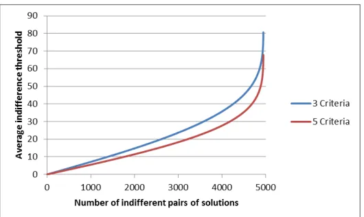
Then we could compute the minimal value and the maximal value of the threshold corresponding to some given number of pairs of alternatives being indifferent. We repeated this 1000 times based on different random numbers, for the case of three and five objectives. The results are summarized in Ta-ble 1. As can be seen, already for relatively small values of the threshold, a relatively large number of pairs of solutions become indifferent. For example, with three criteria, on average, a value of the threshold just slightly greater than 1% of the scale length is enough to have 150 indifferent pairs of alter-natives, and with five criteria, again on average, already a threshold slightly greater than 0.8% is sufficient. This demonstrates the importance of taking indifference into account, because otherwise, there is the risk to misrepre-sent a DM’s preference statements of pairs of alternatives for which there is no clear advantage of one over the other. Further evidence in this sense is given by Figure 1 showing for each number of pairs of indifferent alternatives the corresponding average threshold obtained in the same sequence of 1000 random data sets used for Table 1.
Table 1: Average values and standard deviations of the minimal and maximal threshold
δcorresponding tocicouples of indifferent alternatives in case of 100 alternatives, with 3 criteria and 5 criteria (the values are expressed in percentage of the scale length)
ci20 ci80 ci100 ci150 ci200 ci300 ci400 ci500
minδ maxδ minδ maxδ minδ maxδ minδ maxδ minδ maxδ minδ maxδ minδ maxδ minδ maxδ
3 criteria mean 0.139 0.034 0.559 0.086 0.699 0.104 1.053 0.146 1.410 0.188 2.119 0.27 2.827 0.352 3.537 0.43
std 0.146 0.035 0.566 0.087 0.706 0.105 1.060 0.147 1.417 0.189 2.116 0.271 2.834 0.353 3.543 0.43 5 criteria mean 0.109 0.028 0.438 0.065 0.549 0.078 0.822 0.11 1.095 0.139 1.642 0.195 2.192 0.258 2.743 0.316
std 0.114 0.029 0.443 0.066 0.555 0.079 0.827 0.11 1.101 0.139 1.648 0.196 2.198 0.258 2.748 0.317
2.4. Procedures for optimizing preference elicitation
Figure 1: Average value of the indifference threshold δ on the y axis; given number of pairs of indifferent alternatives on x axis; 100 alternatives with 1000 random data sets. The scale for value functionU is [0,100].
the weighted sum with equal weights or rank ordered centroid, showing that the latter gives a good approximation of the DM’s preferences. Other rules based on the use of incomplete information are discussed in [28, 41, 42]. Other procedures try to propose the DM queries that permit to cut max-imally the space of the parameters in the selected preference model (very often weights of a value function expressed in terms of a weighted sum (2) (see e.g. [18, 26, 47])). Other approaches try to propose queries for which it is maximal the expected reduction of the entropy in the space of the value functions compatible with the preferences expressed by the DM [1, 48]. Other procedures propose questions based on the minimization of the maximum re-gret being the worst-case loss when recommending an alternative a instead of another alternative b ([7, 50]; for an application of this approach to a value function expressed as a Choquet integral see [6]). Finally, another approach recently proposed, considers heuristics based on necessary prefer-ences obtained by robust ordinal regression and pairwise preference indices and ranking acceptability indices obtained by SMAA [11]. Our contribution is in the same spirit of this last approach, with an important difference being that we focus on choice problem rather than on ranking problem.
3. Robust Ordinal Regression allowing for indifference
to assume that every DM has a personal, unknown “precision threshold” δT,
and is indifferent between two alternatives if and only if |U(x)−U(y)| ≤δT. We want to extend ROR to allow the DM to actually declare indifference in such cases, avoiding errors from a forced preference decision. SinceδT is not
known, the new ROR approach allowing for indifference, that we call RORi, has to learn the possible δT along with the possible utility functions U.
In the following, we define a number of concepts that will be helpful in characterizing solutions under the RORi framework. We also, where possible, explain how these characteristics may be checked. For certain classes of user preference models, the mathematical programs that we provide below are simple Linear Programs and can be evaluated efficiently. This is true for example for linear preference models, the two-additive Choquet integral, the Cobb-Douglas utility model or the monotonic additive utility model. If not stated otherwise, we shall assume this situation and will therefore call our mathematical programs “LPs” even if they can be generalized to the nonlinear case.
Let A denote the set of available alternatives and P the set of pairwise preferences and indifferences elicited from the DM so far, where a relation (a b) ∈ P means the DM has stated that a is preferred over b, and (a∼b)∈P represents an indifference statement. We assume A to be finite.
Definition 1 (Possibly acceptable). A solution x is called possibly ac-ceptable if there is at least one (U, δ) compatible with user preference infor-mation P such that ∀y∈A\ {x}: U(x)≥U(y)−δ.
A solutionxis possibly acceptable if and only if the following mathemat-ical program LP1(x) returns a solution valueε >0:
maxε, s.t.
U(x)≥U(y)−δ ∀y∈A\ {x}
U(a)≥U(b) +δ+ε ∀(ab)∈P
|U(a)−U(b)| ≤δ ∀(a∼b)∈P
δ ≥0 EAF
Therein, the decision variables are the parameters defining the utility U, plus the variables δ and ε. Note that the third constraint is equivalent to
Definition 2 (Necessarily acceptable). A solutionxis callednecessarily acceptable if for all(U, δ)compatible with user preference informationP and
∀y∈A\ {x}: U(x)≥U(y)−δ.
It is not so easy to determine whether a solutionx is necessarily accept-able. We have to make sure that there does not exist any triple (U, δ, y) such that U(x) < U(y)−δ. But for this, we have to compare x with each y∈A\ {x} individually using a separate LP. For specifying how this can be done, we start by defining the following binary relation: Solution x is called
possibly preferred overy if and only if there is a (U, δ) compatible with user preference information such that U(x) > U(y) +δ. This is the case if and only if the following LP2(x, y) returns a solution value ε >0:
maxε, s.t.
U(x)≥U(y) +δ+ε
U(a)≥U(b) +δ+ε ∀(ab)∈P
|U(a)−U(b)| ≤δ ∀(a∼b)∈P
δ ≥0 EAF
For abbreviation, let us write LP2(x, y)>0 if LP2(x, y) returns a solution value ε > 0, and LP2(x, y) ≤ 0 if it returns a solution value ε ≤ 0 or is infeasible. Obviously, a solution x isnecessarily acceptable if and only if for eachy∈A\ {x}, solutiony is not possibly preferred overx. This is the case if and only if LP2(y, x)≤0 for ally∈A\ {x}(there is no compatible utility function that strictly prefers y).
Of course it can happen that neither x is possibly preferred over y nor vice versa which brings to the following definition:
Definition 3 (Necessarily indistinguishable). Two solutionsxandyare
necessarily indistinguishable if and only if for all (U, δ) compatible with user preference information P it holds that |U(x)−U(y)| ≤δ.
This can again be checked by using the above LP2: x and y are necessarily indistinguishable if and only if both LP2(x, y)≤0 and LP2(y, x)≤0.
Definition 4 (Possibly best). A solution x is calledpossibly best if there is at least one (U, δ)compatible with user preference information P such that
In other words, solutionx is possibly best if the following mathematical program LP3(x) returns a solution value ε >0:
maxε, s.t.
U(x)≥U(y) ∀y∈A\ {x}
U(a)≥U(b) +δ+ε ∀(ab)∈P
|U(a)−U(b)| ≤δ ∀(a∼b)∈P
δ ≥0 EAF
Definition 5 (Necessarily best). A solutionxis called necessarily bestif for all(U, δ)compatible with user preference informationP and∀y∈A\{x}: U(x)≥U(y).
Similarly to necessarily acceptable, determining whether a solution xis nec-essarily best is computationally demanding.
Definition 6 (Possibly globally preferred). A solution x is called pos-sibly globally preferred if there is at least one (U, δ) compatible with user preference information P such that ∀y∈A\ {x}: U(x)> U(y) +δ.
The followingLP4(x) determines whether a solutionxis possibly globally preferred, which is the case if and only if LP4(x) returns a solution value ε >0:
maxε, s.t.
U(x)≥U(y) +δ+ε ∀y∈A\ {x}
U(a)≥U(b) +δ+ε ∀(ab)∈P
|U(a)−U(b)| ≤δ ∀(a ∼b)∈P
δ≥0 EAF
Definition 7 (Necessarily globally preferred). A solutionxis called nec-essarily globally preferred if for all (U, δ) compatible with user preference information P and ∀y∈A\ {x}: U(x)> U(y) +δ.
To define our goal, we assume the DM has an underlying true utility function UT and true precision threshold δT (please note that we do not assume the DM is aware of it, only that it exists). Then, the above definitions can be adapted and a solution x is considered
• (truly) acceptable, if UT(x)≥UT(y)−δT for all y∈A,
• (truly) best, if UT(x)≥UT(y) for ally ∈A.
Two solutionsx, yare called(truly) indistinguishable, if|UT(x)−UT(y)| ≤ δT.
The selection problem addressed in this paper may then have two possible goals:
• Goal A:Identifyall solutions truly acceptable to the DM, i.e., all xsuch that there is no y with UT(y) > UT(x) + δT. This gives the DM the maximal choice of solutions to choose from, which is particularly useful if there are other, secondary criteria that are not explicitly modelled.
• Goal B: Identify at least one solution truly acceptable to the DM, i.e., at least onexsuch that there is noywithUT(y)> UT(x) +δT. While this
may generate a smaller set of acceptable solutions compared to Goal A, it is expected to converge faster since it can discard solutions more quickly as long as at least one acceptable solution remains.
In the following, we will present ways to reach those goals efficiently.
4. Algorithms
RORi iteratively presents pairs of alternatives (x, y) to the DM and asks whether the DM prefers x, prefers y, or is indifferent. At any point in time, the algorithm maintains a list S ⊆ A of candidate solutions which is guar-anteed to include a solution acceptable to the DM based on the information elicited so far. By eliciting more and more information, the size of this set reduces until there is only one solution left or it is clear that all remaining solutions are necessarily indistinguishable, and the algorithm terminates.
Obviously, the size of S in each iteration and the number of preference elicitations required before the algorithm terminates depend on the pairs of solutions shown to the DM. So, the natural question arises exactly which pair of solutions should be shown to the DM in each iteration such that the expected number of required preference elicitations is minimized. This will be discussed in Section 5.
4.1. Identifying all truly acceptable solutions
Algorithm 1 shows the general algorithmic framework that will identify
all solutions that areacceptable to the DM, i.e., all xsuch that there is no y with UT(y)> UT(x) +δT.
Algorithm 1 Finding all truly acceptable solutions
1: Identify the set of possibly acceptable solutions S using LP1 for each solution.
2: Search for a pair (x, y) (x, y ∈ S) of solutions that have not yet been shown to the DM and that are not necessarily indistinguishable (tested by LP2).
3: If such a pair is found, show it to the DM, update the constraints ac-cordingly, and go to Step 1.
4: Otherwise stop and return setS.
Proposition 4.1. If the true utility function UT is contained in the set U
of utility functions defined by the preference model EAF, then Algorithm 1
terminates with the set of all truly acceptable solutions.
Proof. LetU(k)denote the set of all pairs (U, δ) such that (U, δ) is compatible
with the preference information P(k) present at the beginning of the k-th iteration of the algorithm: (U, δ) ∈ U(k) if and only if U(a) > U(b) + δ
∀(a b) ∈ P(k) and |U(a)−U(b)| ≤ δ ∀(a ∼ b) ∈ P(k). We always have
(UT, δT) ∈ U(k), since the DM never declares a preference information that
is inconsistent with his true (U, δ). Let now x be acceptable, i.e., UT(x) ≥
UT(y)− δT for all y ∈ A. Then, because (UT, δT) ∈ U(t), x is possibly
Conversely, assume that y ∈ A is not acceptable, i.e., there is a w ∈ A such that UT(w) > UT(y) +δT. Let x denote a truly best solution (which must exist in view of the finiteness of A), i.e. a solution withUT(x)≥UT(z) for all z ∈A. In particular,
UT(x)≥UT(w)> UT(y) +δT. (10)
Equation (10) implies together with
UT(a)> UT(b) +δ ∀(ab)∈P(k)
|UT(a)−UT(b)| ≤δ ∀(a∼b)∈P(k) )
that the constraints of LP2(x, y) are satisfied for someε >0, and so we have LP2(x, y)>0. The termination condition of Algorithm 1 entails that in the last iterationt, either (i) (x, y) has already been shown to the DM before, or (ii) LP2(x, y)≤0 and LP2(y, x)≤0.
Since LP2(x, y)>0 as demonstrated above, (x, y) must have been shown to the DM in a previous iteration k < t. In view of (10), the DM has stated x y, so the constraint U(x) > U(y) +δ must have been added to the set of constraints. As a consequence, y is not possibly acceptable in iteration t anymore and is therefore not contained in the final solution set.
4.2. Identifying at least one truly acceptable solution
Identifying all acceptable solutions as described in the previous subsection provides the DM with some choice. However, we may be able to converge quicker and to a smaller set if we aim at identifying the true best rather than all acceptable solutions. Unfortunately, identifying the DM’s true best solution may not always be possible. If there are other solutions that are within the DM’s precision threshold, then we may not be able to conclude which solution is best, simply because the DM would not be able to rank these solutions. The following Algorithm 2 thus finds a subset of acceptable solutions that is guaranteed to include the true best solution. The only difference between Algorithm 2 and Algorithm 1 is that in each iteration, the current set S is determined to include all possibly best solutions rather than all possibly acceptable solutions.
Proposition 4.2. If the true utility function UT is contained in the set U
of utility functions defined by the preference model EAF, then Algorithm 2
Algorithm 2 Finding at least one acceptable solution
1: Identify the set of possibly best solutions S using LP3 for each solution.
2: Search for a pair (x, y) (x, y ∈ S) of solutions that have not yet been shown to the DM and that are not necessarily indistinguishable (tested by LP2).
3: If such a pair is found, show it to the DM, update the constraints ac-cordingly, and go to Step 1.
4: Otherwise stop and return setS.
(a) Each truly best solution is contained in S.
(b) The solutions in S are pairwise truly indistinguishable:
|UT(x)−UT(y)| ≤δT for all x, y ∈S.
Proof. To show (a), let x be truly best. With U(t) defined analogously
to the proof of Proposition 1, we have again (UT, δT) ∈ U(t) in the final
iteration t. Therefore, solution x is possibly best in iteration t and thus passes the test in Step 1 of Algorithm 2 in this iteration. As a consequence, x is contained in the final set S. To show (b), let us consider two different solutions x, y ∈ S. According to the termination condition of Algorithm 2, either (x, y) has already been shown to the DM before, or
LP2(x, y)≤0 and LP2(y, x)≤0. (11)
In the first case where (x, y) has already been shown in some previous itera-tion k < t, the DM can only have stated indifference, since if he/she would have stated (say) x y, then the constraint U(x) > U(y) +δ would have been added to the set of constraints, with the consequence that y would not have passed the test in Step 1 of iterationt, being not possibly best anymore. So there remains only the case that iteration t produces (11). In this case, however, x and y are necessarily indistinguishable based on the information present in iteration t, i.e., |U(x)−U(y)| ≤ δ ∀(U, δ) ∈ U(t). In particular,
because of (UT, δT)∈ U(t), this implies |UT(x)−UT(y)| ≤δT.
solution set in the previous iteration k−1. The following result provides a positive answer to this question.
Proposition 4.3. If in the call of LP3 by the k-th iteration of Algorithm 2, the constraintU(x)≥U(y) ∀y ∈A\ {x}is replaced by the constraint U(x)≥
U(y) ∀y∈S(k−1)\ {x}, where S(`) denotes the set of solutions as produced in
iteration ` of the algorithm, then the feasible set of LP3 remains unchanged, and therefore the same set of possibly best solutions x is produced in this iteration.
Proof. Let A∗U denote the set of possibly best solutions with respect to preference information U, and letU(k) be defined analogously to the proof of
Proposition 1. ThenS(k−1) =A∗U(k−1). First, we show that for each preference information U on A, for each fixed (U, δ) ∈ U and for each fixed x∈A, the condition
U(x)≥U(y) ∀y∈A∗U \ {x} (12) implies
U(x)≥U(y) ∀y ∈A\ {x}. (13) Indeed, assume that (12) holds, but that (13) is violated for some y, i.e., U(x) < U(y). Let z∗ ∈ arg maxz∈A\{x}U(z). Then U(y) ≤ U(z∗), hence U(x) < U(z∗), and z∗ is obviously possibly best with respect to U, that is, z∗ ∈A∗U \ {x}. This contradicts (12).
To show the statement of the Proposition, we consider now an iterationk and some fixed x ∈ A. In iteration k, the constraints of LP3 restrict the feasible set to (U, δ) ∈ U(k). Since the constraints are extended in each
iteration of Algorithm 2, we have U(k) ⊆ U(k−1). Thus, in the call of LP3 in
iteration k for the given x, each solution (U, δ) that is feasible with respect to the second and the third type of constraints, also satisfies the condition (U, δ)∈ U(k−1). Consequently, if for such a pair (U, δ), the inequality
U(x)≥U(y) ∀y∈A∗U(k−1)\ {x} (14)
corresponding to (12) holds, we can apply the auxiliary result from above withU =U(k−1)and conclude that (13) is valid, and therefore (U, δ) is feasible
5. Heuristics to speed up convergence
In the above, we have simply restricted the questions (or pairs of solu-tions) to be shown to the DM to those pairs that are guaranteed to provide new information. In the following, we consider some heuristics to pick a pair among all the “reasonable” pairs of solutions. Denote by S the set of pairs of solutions in (S ×S) that have not yet been shown to the DM and that are not necessarily indistinguishable at any stage in the interaction process (this set gets smaller and smaller over the course of the interaction, but we use the same symbol in all iterations in order to simplify notation).
The benchmark will be the following simple approach H1.
H1 Pick a pair randomly among all the pairs in S.
The following heuristic H2 always maintains the solution cidentified by the DM as the best so far, and compares it to the solution in S that could possibly be preferred overcby the largest margin across all compatible value functions. This method has been proposed in [4].
H2 The first pair of solutions is picked randomly from S. Let us denote by c the solution preferred by the DM (one at random in case of in-difference). In subsequent iterations, present the pair (x, c) ∈ S with x = argmax LP2(x, c). If the DM prefers x, the best so far solution c is set to x.
H3 picks pairs of solutions that can have maximal contradiction in values based on the set of compatible value functions.
H3 Pick the pair (x, y)∈ S as (x, y) = argmax{LP2(x, y) +LP2(y, x)}.
H4 uses the most discriminative value function in the spirit of [35] as a best guess of the DM’s true value function, and then shows the DM the presumed best and second best solution. The hope is that if the DM confirms the presumed ordering, it would also be possible to remove many other solutions from S.
maxε, s.t.
U(a)≥U(b) +δ+ε ∀(ab)∈P
|U(a)−U(b)| ≤δ−ε ∀(a∼b)∈P
δ ≥0 EAF
H4 Identify the most discriminative value function (Ud, δd) by solving LP5
above. Then, show the DM the pair of solutions consisting of the best and second best solution according to Ud.
The common idea behind H5, H6 and H7 is to look one step ahead. For each possible pair (x, y) ∈ S, these heuristics consider the three possible responses of the DM: x y, x ≺ y, x ∼ y. H5 minimizes the number of remaining possibly acceptable solutions in the worst case, whereas H6 min-imizes the expected number of the remaining possibly acceptable solutions. H7 looks at the expected resulting entropy, where entropy of a decision sit-uation has been defined in [48] and can be calculated based on a number of value functions (U, δ) compatible with preference information. In particular, the entropy E given a set of solutions S and a finite sample set of utility functions U is defined as
E(S,U) =−X
x∈S
pxlogpx (15)
where px is the fraction of utility functions inU for which solution xis best.
To calculate the expected value in H6 and H7, it is necessary to assign probabilities to the three possible responses of the DM. We do this by gener-ating 10,000 random utility functions compatible with the elicited preference information using the algorithm by [45, 46]. Then the probability that the DM will select x y, x≺ y, or x∼ y is estimated by the fraction of utility functions that would result in the respective decision.
H5 For each pair (x, y)∈ S
– P2 Add the constraint U(y) ≥ U(x) +δ + ε to LP1 and determine the number of solutions that can be still possibly acceptable solutions, denoted by P Pxy≺,
– P3Add the constraint|U(y)−U(x)| ≤δto LP1 and determine the num-ber of solutions that can be still possibly acceptable solutions, denoted byP Pxy∼.
Pick the pair (x, y) that minimizes the number of possibly acceptable so-lutions in the worst case, i.e., (x, y) = argmin(x,y)max{P Pxy, P Pxy≺, P Pxy∼}
H6 For each pair (x, y)∈ S
– P1Add the constraintU(x)≥U(y) +δ+εto LP1 and check how many solutions can be still possibly best solutions, denoted by P Pxy,
– P2Add the constraintU(y)≥U(x) +δ+εto LP1 and check how many solutions can be still possibly best solutions, denoted by P Pxy≺,
– P3 Add the constraint|U(y)−U(x)| ≤δ to LP1 and check how many solutions can be still possibly best solutions, denoted by P Pxy∼,
– P4 Generate a set of utility functions (U, δ) compatible with the pref-erence information. Determine what fraction of those utility functions would preferx, prefer y, or be indifferent (pxy, p≺xy, p∼xy).
Pick the pair (x, y) that minimizes the expected number of possibly best solutions, i.e., (x, y) = argmin(x,y){pxy ·P Pxy +p≺xy·P Pxy≺ +p∼xy·P Pxy∼}.
H7 For each pair (x, y)∈ S
– P1Add the constraintU(x)≥U(y) +δ+εto LP3 and check how many solutions can be still be possibly best solutions, denoted by P Bxy,
– P2Add the constraintU(y)≥U(x) +δ+εto LP3 and check how many solutions can be still possibly best solutions, denoted by P Bxy≺,
– P3 Add the constraint|U(y)−U(x)| ≤δ to LP3 and check how many solutions can be still possibly best solutions, denoted by P Bxy∼,
– P4 Generate a set of utility functions (U, δ) ∈ U compatible with the preference information. Determine what fraction of those utility func-tions would prefer x, prefer y, or be indifferent, (pxy, p≺xy, p∼xy). Also calculate the entropy of the resulting decision situations
Pick the pair (x, y) that minimizes the expected entropy of the resulting decision situation, i.e., (x, y) = argmin{pxy·Exy +pxy≺ ·Exy≺ +p∼xy·Exy∼}.
Note that H5, H6 and H7 as described above require to solve 3 LPs for every pair of solutions still in S that has not yet been shown to the DM, which makes the algorithm rather slow. In the computational experiments reported below, we have thus replaced the solution of the LPs by a numerical approximation based on the 10,000 random compatible utility functions that we require anyway to estimate probabilities in H6 and H7. In particular, for each considered pair of solutions and possible DM preference (xy, x ≺y, orx∼y), we remove the utility functions that are no longer compatible with the presumed new preference information and simply check how many solu-tions are still acceptable or best for at least one of the remaining preference functions. A limited number of experiments indicated that this is computa-tionally much faster and even works slightly better, presumably because it ignores cases where a solution would only be acceptable or best by a tiny fraction of compatible utility functions.
6. Empirical results
6.1. Experimental setup
For our experiments, we need an artificial decision maker, and we assume the two-additive Choquet preference model as the DM’s internal model. Our artificial decision maker answers to preference elicitations in terms of pair-wise comparisons according to this underlying utility function (UT, δT), that
is of course otherwise unknown to the elicitation algorithms. For every ex-periment, we average over 50 problem instances, using the same problem instances across algorithms. First, we generate random weights for the dif-ferent attributes, resulting in a linear utility function of the artificial DM. For each problem instance, we randomly generate the desired number of mu-tually non-dominated alternatives in real-valued attribute space. Then, the artificial DM’s discrimination thresholdδT is determined such that we obtain
Table 2: Average number and standard error of required DM interactions until the al-gorithm terminates with a subset of all acceptable solutions including the best one, for
N = 100 andP ={20,80,150}indifferent pairs and m= 3 criteria.
P H0 H1 H2 H3 H4 H5 H6 H7 20 99 13.98 16.64 13.94 16.78 12.28 10.96 18.0
±0 ±0.34 ±0.62 ±0.41 ±0.52 ±0.30 ±0.29 ±0.55
80 99 13.96 16.32 13.74 16.56 12.28 10.56 17.52
±0 ±0.34 ±0.63 ±0.43 ±0.52 ±0.31 ±0.31 ±0.61
150 99 13.5 16.3 13.66 16.56 12.08 10.54 17.16
±0 ±0.38 ±0.62 ±0.43 ±0.52 ±0.33 ±0.29 ±0.64
As an additional benchmark to demonstrate the benefit of using RORi and our heuristics to pick pairs of solutions to show to the DM we also include the following straightforward algorithm to determine at least one acceptable solution: go through the solutions in a random sequence, initialise the first solution as the current best and compare each solution in turn with the current best, making the challenger the current best only if the challenger is preferred. This simple algorithm is guaranteed to identify an acceptable solution but obviously requires N −1 pairwise comparisons, whereN is the number of alternatives to choose from. It is denoted as H0 in the tables below.
6.2. Comparison of elicitation heuristics
For the baseline experiments reported in this section, we use Algorithm 2 as the general framework, N = 100 alternatives, m = 3 attributes and P =
{20,80,150} pairs of solutions being indifferent. The average number of required DM interactions until the algorithm terminates is summarized in Table 2.
Clearly, all methods are much more efficient than the above mentioned simple approach that would require 99 pairwise comparisons.
Table 3: Percentage of DM interactions that result in an indifference statement, for Algo-rithm 2,N = 100, P={20,80,150} indifferent pairs andm= 3 criteria.
P H0 H1 H2 H3 H4 H5 H6 H7 20 0.08% 0.29% 0.24% 0.00% 0.12% 0.33% 0.55% 0.00% 80 0.46% 2.01% 0.74% 1.75% 1.93% 1.95% 3.60% 0.57% 150 0.95% 4.15% 1.47% 3.37% 2.90% 4.80% 6.07% 1.63
heuristic H7 based on look-ahead and entropy calculation, presumably be-cause minimizing entropy is not very well aligned with our goal of minimizing the number of interactions.
Only two of the look-ahead heuristics, namely H5 and H6, are signifi-cantly better than random selection. Of the two, the method that greedily minimizes the expected number of remaining solution candidates (H6) works much better than H5 which minimizes the number of remaining solution can-didates in the worst case. Although H6 is computationally more expensive to compute because it needs to estimate the probabilities for the DM’s re-sponse, this extra effort seems to pay off. H6 requires between 21.6% and 24.3% less interactions than the random selection of pairs.
Table 3 reports on the percentage of interactions with the DM that result in an indifference statement. This percentage is roughly in the ballpark of the percentage of all possible pairwise comparisons for 20, 80 and 150 indifferent pairs, which is 0.4%, 1.6%, 3.0% for 100 alternatives. H7 based on entropy and H0 create the smallest percentage of indifference responses for P = 20, and P ={80,150}, respectively, whereas Random (H1), H5 and H6 create relatively many indifference responses.
6.3. Identifying all acceptable solutions
Table 4: Average number and standard error of required DM interactions until the algo-rithm terminates with the set of all acceptable solutions, for N = 100, P ={20,80,150} indifferent pairs andm= 3 criteria.
P H1 H2 H3 H4 H5 H6 H7 20 16.58 18.06 17.36 20.72 13.26 11.46 19.66
±0.45 ±0.65 ±0.57 ±0.88 ±0.29 ±0.31 ±0.63
80 16.74 18.08 17.96 21.14 13.5 11.44 19.2
±0.46 ±0.67 ±0.69 ±0.93 ±0.33 ±0.31 ±0.67
150 16.8 18.14 18.4 21.04 13.4 11.58 19.12
±0.46 ±0.67 ±0.70 ±0.93 ±0.34 ±0.30 ±0.71
Table 5: Percentage of DM interactions that result in an indifference statement, for Algo-rithm 1,N = 100, P={20,80,150} indifferent pairs andm= 3 criteria.
P H1 H2 H3 H4 H5 H6 H7 20 0.7% 0.2% 0.5% 0.3 % 0.5% 0.5% 0% 80 2.7% 0.9% 2.1% 1.6% 1.9% 5.2% 0% 150 5.2% 1.8% 3.9% 2.8% 3.9% 6.6% 1.8%
6.4. Influence of the number of alternatives
In this section, we examine the influence of the number of alternatives on the required number of preference elicitations. In addition to N = 100, we examine N = 50 and N = 200. The number of criteria is still 3, and we choose δT in a way that results in 1.6% indifferences, i.e., 20, 80 and 320 indifferent pairs for 50, 100 or 200 alternatives, respectively. Because many of the heuristics resulted in performances worse than random selection, we only consider H1, H5, and H6 here in addition to the straightforward benchmark H0 (see Table 6(a)).
The number of preference elicitations seems to be roughly linear. A linear regression for the H6 heuristic results in 9.29 + 0.018N which means that for each additional alternative, the number of expected required preference elicitations only increases by about 0.02.
6.5. Influence of the number of criteria
[image:28.612.113.403.319.378.2]Table 6: Average number and standard error of required DM interactions until the algo-rithm terminates with a set of acceptable solutions,...
(a) ...for different numbers of alterna-tivesN, indifference in 1.6% of all pos-sible pairs andm= 3 criteria.
N H0 H1 H5 H6
50 49 12.32 10.92 9.86
±0 ±0.27 ±0.26 ±0.24
100 99 13.96 12.28 10.56
±0 ±0.34 ±0.31 ±0.31
200 199 15.0 13.20 11.64
±0 ±0.37 ±0.34 ±0.30
(b) ...for different numbers of criteria
mand indifference inP= 80 pairs.
m H0 H1 H5 H6
3 99 13.96 12.28 10.56
±0 ±0.34 ±0.31 ±0.31
5 99 33.38 35.02 27.64
±0 ±0.60 ±0.73 ±0.53
and identification of the best solution. Again, we only consider the most promising heuristics.
As can be seen from Table 6(b), the necessary number of pairwise compar-isons increases sharply with the number of criteria. The reason is probably that the preference model has more parameters, and requires more infor-mation in terms of preference elicitations before it is accurate enough to be helpful in pruning solutions from the set of possibly best solutions. The rel-ative performance, however, remains similar, and H6 is still able to reduce the number of preference elicitations by 17.2% compared to RORi with ran-dom selection (24.4% for the 3 criteria case), and by 72.1% compared to the default heuristic H0 (89.3% for the 3 criteria case).
7. Discussion and Conclusions
comparisons compared to an algorithm that considers all alternatives in turn and always keeps the best-so-far — even when the pairs of solutions shown to the DM are picked randomly. The reduction is lower if the number of criteria is higher, because the model then has more parameters and thus more information is needed to derive meaningful parameter values. Similarly, the reduction is higher with a higher number of alternatives, because the savings are low initially but grow with the number of alternatives evaluated as the model becomes more and more precise.
Regarding the proposed heuristics to decide which pair of solutions to show to the DM, surprisingly, most heuristics, including those we took from the literature, perform worse than random sampling when evaluated based on the number of preference elicitations needed to complete the selection. The best heuristic uses a sophisticated one-step look-ahead technique, which on the problems considered further reduces the necessary number of samples by about 20% compared to RORi with random selection of pairs. Together, depending on the test problem, our method saves about 90% of the required pair-wise preference elicitations compared to a simple algorithm that consid-ers all alternatives in turn and always keeps the best-so-far.
There are various avenues for future work. While we have used the Cho-quet integral as preference model in this paper, an extension to other pref-erence models should be straightforward. More heuristics can be developed, and should be tested on a wider range of benchmark problems. Finally, one may consider showing the DM not only pairs of existing alternatives, but also fictitious alternatives in order to speed up convergence.
Acknowledgments
The second and the third authors wish to acknowledge the funding by the “FIR of the University of Catania BCAEA3, New developments in Mul-tiple Criteria Decision Aiding (MCDA) and their application to territorial competitiveness”.
References
[2] S. Angilella, S. Greco, F. Lamantia, and B. Matarazzo. Assessing non-additive utility for multicriteria decision aid. European Journal of Op-erational Research, 158(3):734–744, 2004.
[3] S. Angilella, S. Corrente, and S. Greco. Stochastic multiobjective ac-ceptability analysis for the Choquet integral preference model and the scale construction problem. European Journal of Operational Research, 240(1):172–182, 2015.
[4] N. Argyris, A. Morton, and J.R. Figueira. CUT: A multicriteria ap-proach for concavifiable preferences. Operations Research, 62(3):633– 642, 2014.
[5] F.H. Barron and B.E. Barrett. Decision quality using ranked attribute weights. Management Science, 42(11):1515–1523, 1996.
[6] N. Benabbou, C. Gonzales, P. Perny, and P. Viappiani. Minimax regret approaches for preference elicitation with rank-dependent aggregators.
EURO Journal on Decision Processes, 3(1-2):29–64, 2015.
[7] C. Boutilier, R. Patrascu, P.l Poupart, and D. Schuurmans. Constraint-based optimization and utility elicitation using the minimax decision criterion. Artificial Intelligence, 170(8):686–713, 2006.
[8] J. Branke, S. Corrente, S. Greco, and W.J. Gutjahr. Using indifference information in robust ordinal regression. In International Conference on Evolutionary Multi-Criterion Optimization, pages 205–217. Springer, 2015.
[9] A. Chateauneuf and J.Y. Jaffray. Some characterizations of lower prob-abilities and other monotone capacities through the use of M¨obius in-version. Mathematical Social Sciences, 17:263–283, 1989.
[10] G. Choquet. Theory of capacities. Annales de l’institut Fourier, 5(54): 131–295, 1953.
[12] S. Corrente, S. Greco, M. Kadzi´nski, and R. S lowi´nski. Robust ordinal regression in preference learning and ranking. Machine Learning, 93 (2-3):381–422, 2013.
[13] S. Corrente, S. Greco, M. Kadzi´nski, and R. S lowi´nski. Robust ordinal regression. Wiley Encyclopedia of Operations Research and Management Science, pages 1–10, 2014.
[14] S. Corrente, S. Greco, and A. Ishizaka. Combining analytical hierarchy process and Choquet integral within non-additive robust ordinal regres-sion. Omega, 61:2–18, 2016.
[15] M. Ehrgott, J.R. Figueira, and S. Greco (eds.). Trends in Multiple Criteria Decision Analysis. Springer, New York, 2010.
[16] P.C. Fishburn. Interval representations for interval orders and semiorders. Journal of Mathematical Psychology, 10(1):91–105, 1973.
[17] P.C. Fishburn. Interval orders and interval graphs: A study of partially ordered sets. John Wiley & Sons, 1985.
[18] K. Gajos and D.S. Weld. Preference elicitation for interface optimiza-tion. In Proceedings of the 18th annual ACM symposium on User inter-face software and technology, pages 173–182. ACM, 2005.
[19] A. Giarlotta and S. Greco. Necessary and possible preference structures.
Journal of Mathematical Economics, 49(2):163 – 172, 2013.
[20] I. Gilboa and D. Schmeidler. Additive representations of non-additive measures and the Choquet integral. Annals of Operations Research, 52: 43–65, 1994.
[21] M. Grabisch. The application of fuzzy integrals in multicriteria decision making. European Journal of Operational Research, 89:445–456, 1996.
[22] M. Grabisch. k-order additive discrete fuzzy measures and their repre-sentation. Fuzzy Sets and Systems, 92:167–189, 1997.
[24] S. Greco, V. Mousseau, and R. S lowi´nski. Ordinal regression revisited: multiple criteria ranking using a set of additive value functions.European Journal of Operational Research, 191(2):416–436, 2008.
[25] S. Greco, R. S lowi´nski, J.R. Figueira, and V. Mousseau. Robust ordinal regression. In M. Ehrgott, J.R. Figueira, and S. Greco, editors, Trends in Multiple Criteria Decision Analysis, pages 241–283. Springer, 2010.
[26] V.S. Iyengar, J. Lee, and M. Campbell. Evaluating multiple attribute items using queries. In Proceedings of the 3rd ACM conference on Elec-tronic Commerce, pages 144–153. ACM, 2001.
[27] E. Jacquet-Lagr`eze and Y. Siskos. Assessing a set of additive utility functions for multicriteria decision-making, the UTA method. European Journal of Operational Research, 10(2):151–164, 1982.
[28] M. Kadzi´nski and M. Michalski. Scoring procedures for multiple criteria decision aiding with robust and stochastic ordinal regression.Computers & Operations Research, 71:54–70, 2016.
[29] M. Kadzi´nski and T. Tervonen. Robust multi-criteria ranking with addi-tive value models and holistic pair-wise preference statements. European Journal of Operational Research, 228(1):169–180, 2013.
[30] R.L. Keeney and H. Raiffa. Decisions with multiple objectives: Prefer-ences and value tradeoffs. J. Wiley, New York, 1976.
[31] R. Lahdelma and P. Salminen. SMAA-2: Stochastic multicriteria ac-ceptability analysis for group decision making. Operations Research, 49 (3):444–454, 2001.
[32] R. Lahdelma, J. Hokkanen, and P. Salminen. SMAA-Stochastic Multi-objective Acceptability Analysis. European Journal of Operational Re-search, 106(1):137–143, 1998.
[33] R.D. Luce. Semiorders and a theory of utility discrimination. Econo-metrica, 24(2):178–191, 1956.
[35] S. Phelps and M. K¨oksalan. An interactive evolutionary metaheuristic for multiobjective combinatorial optimization. Management Science, 49 (12):1726–1738, 2003.
[36] M. Pirlot and P. Vincke. Semiorders: properties, representations, appli-cations. Springer Science & Business Media, 2013.
[37] G.C. Rota. On the foundations of combinatorial theory I. Theory of M¨obius functions. Wahrscheinlichkeitstheorie und Verwandte Gebiete, 2:340–368, 1964.
[38] B. Roy. Multicriteria Methodology for Decision Aiding. Kluwer Aca-demic, Dordrecht, 1996.
[39] B. Roy. Paradigm and Challenges. In S. Greco, J.R. Figueira, and M. Ehrgott, editors, Multiple Criteria Decision Analysis: State of the Art Surveys, pages 19–39. Springer, Berlin, 2016.
[40] B. Roy, J.R. Figueira, and J. Almeida-Dias. Discriminating thresholds as a tool to cope with imperfect knowledge in multiple criteria decision aiding: Theoretical results and practical issues. Omega, 43:9–20, 2014.
[41] A.A. Salo and R.P. H¨am¨al¨ainen. Preference ratios in multiattribute evaluation (prime)-elicitation and decision procedures under incomplete information. IEEE Transactions on Systems, Man, and Cybernetics-Part A: Systems and Humans, 31(6):533–545, 2001.
[42] P. Sarabando and L.C. Dias. Simple procedures of choice in multicrite-ria problems without precise information about the alternatives’ values.
Computers & Operations Research, 37(12):2239–2247, 2010.
[43] G. Shafer. A Mathematical Theory of Evidence. Princeton University Press, 1976.
[44] Y. Siskos, E. Grigoroudis, and N.F. Matsatsinis. UTA methods. In S. Greco, J.R. Figueira, and M. Ehrgott, editors,Multiple Criteria Deci-sion Analysis: State of the Art Surveys, pages 315–362. Springer, Berlin, 2016.
[46] T. Tervonen, G. Van Valkenhoef, N. Bast¨urk, and D. Postmus. Hit-and-run enables efficient weight generation for simulation-based multiple criteria decision analysis. European Journal of Operational Research, 224:552–559, 2013.
[47] O. Toubia, J.R. Hauser, and D.I. Simester. Polyhedral methods for adaptive choice-based conjoint analysis. Journal of Marketing Research, 41(1):116–131, 2004.
[48] G. van Valkenhoef and T. Tervonen. Entropy-optimal weight constraint elicitation with additive multi-attribute utility models. Omega, 64:1–12, 2016.
[49] P.P. Wakker. Additive representations of preferences: A new foundation of decision analysis. Springer, 1989.