©2019 The Authors Journal of the Royal Statistical Society: Series B
(Statistical Methodology) Published by John Wiley & Sons Ltd on behalf of the Royal Statistical Society.
This is an open access article under the terms of the Creative Commons Attribution License, which permits use, distribution and reproduction in any medium, provided the original work is properly cited.
1369–7412/19/81385 81,Part2,pp.385–408
Multiple influential point detection in high
dimensional regression spaces
Junlong Zhao,
Beijing Normal University, People’s Republic of China
Chao Liu and Lu Niu
Beihang University, People’s Republic of China
and Chenlei Leng
University of Warwick, Coventry, and Alan Turing Institute, London, UK
[Received February 2017. Final revision December 2018]
Summary. Influence diagnosis is an integrated component of data analysis but has been severely underinvestigated in a high dimensional regression setting. One of the key challenges, even in a fixed dimensional setting, is how to deal with multiple influential points that give rise to masking and swamping effects. The paper proposes a novel group deletion procedure re-ferred to as multiple influential point detection by studying two extreme statistics based on a marginal-correlation-based influence measure. Named the min- and max-statistics, they have complementary properties in that the max-statistic is effective for overcoming the masking ef-fect whereas the min-statistic is useful for overcoming the swamping efef-fect. Combining their strengths, we further propose an efficient algorithm that can detect influential points with a pre-specified false discovery rate. The influential point detection procedure proposed is simple to implement and efficient to run and enjoys attractive theoretical properties. Its effectiveness is verified empirically via extensive simulation study and data analysis. An R package implement-ing the procedure is freely available.
Keywords: False discovery rate; Group deletion; High dimensional linear regression; Influential point detection; Masking and swamping; Robust statistics
1. Introduction
Recent decades have witnessed an explosion of high dimensional data in applied fields including biology, engineering, finance and many other areas. Given a data set consisting of{Xi,Yi}ni=1
whereYi∈Ris the response andXi∈Rpis the covariate for theith observation, the main interest is often to conduct a regression analysis to relateY toX, the simplest model for which takes the linear form.
A usual assumption in linear regression is that the observations are all generated from the same model. In many applications, however, the data that are collected often contain contaminated or noisy observations due to a plethora of reasons. Those observations exerting great influence on statistical analysis, thus named influential points, can seriously distort all aspects of data analysis such as altering the estimate of the regression coefficient and swaying the outcome of
Address for correspondence: Chenlei Leng, Department of Statistics, University of Warwick, Coventry, CV4
7AL, UK.
statistical inference (Draper and Smith, 2014). Thus, when influential points are present, fitting the model based on a clean data assumption leads to at best a very crude approximation to the model and at worst a completely wrong solution. For fixed dimensional models, we refer the reader to Cook (1977), Belsleyet al. (1980), Chatterjee and Hadi (1986), Imon (2005), Zhuet al. (2007, 2012) and Nurunnabiet al. (2014), among many others. For high dimensional models, Zhaoet al. (2013) found that influential observations could negatively impact many methods that have recently been developed for dealing with high dimensionality, such as the lasso for variable selection (Tibshirani, 1996) and sure independence screening for variable screening (Fan and Lv, 2008).
As a result, influence diagnosis has been long recognized as a central problem in statis-tical analysis. An entire line of research has been devoted to devising robust methods that are less prone to influential observations; see, for example, the books on robust regression by Maronnaet al. (2006), Huber and Ronchetti (2009) and Rousseeuw and Hubert (2011), as well as the papers by Wanget al. (2007) and Fan et al. (2014) for variable selection with heavy-tailed noise and She and Owen (2011) for an outlier robust method for the mean shift model. However, identifying influential points can often be of major scientific interest. For mul-tivariate high dimensional data containing onlyXis, Aggarwal and Yu (2001) proposed to use projection and Filzmoseret al. (2008) and Shieh and Hung (2009) applied principal compo-nent analysis, whereas Roet al. (2015) used a robust covariance matrix estimator for defining distance.
When pis fixed, an attractive measure is to quantify individual observations’ influence in changing the ordinary least squares (OLS) estimator and resulting quantities; see, notably, Cook’s distance (Cook, 1977), Studentized residuals (Velleman and Welsch, 1981), DFFITS (Welsch and Kuh, 1977; Belsleyet al., 1980) and Welsch’s distance (Welsch, 1982). Since these measures are all based on OLS estimation, they are not applicable to high dimensional data. In contrast, the problem of influence diagnosis in high dimensional regression has received little attention, mainly due to the difficulty in establishing a coherent theoretical framework, even in a fixed dimension setting, and a lack of easily implementable procedures. To overcome this, Zhao
et al. (2013) found that influence can be measured by examining how an individual observation affects the marginal correlation between the response and the predictors, which is a ubiquitous quantity in almost all aspects of regression analysis. They proposed a high dimensional influence measure named HIM to flag those points that have a great influence on the calculated value of marginal correlations as influential, in a sense to be defined later. An attractive feature of HIM is that its asymptotic properties can be rigorously established to enable the use of a multiple-testing procedure for detecting influential points.
and van Zomeren, 1990; Hadi and Simonoff, 1993; Imon, 2005; Panet al., 2000; Nurunnabi
et al., 2014; Roberts et al., 2015) but it is currently an open problem for high dimensional problems.
The main aim of this paper is to propose a new procedure for detecting multiple influential points for high dimensional data based on HIM. Via random group deletion, we propose a novel procedure named MIP, short for multiple influential point detection for high dimensional data. Along with the process, we propose two novel quantities named max- and min-statistics to assess the extremeness of each point when data are subsampled. Our theoretical studies show that these two statistics have complementary properties. The min-statistic is useful for overcoming the swamping effect but less effective for masked influential observations, whereas the max-statistic is well suited for detecting masked influential observations but is less effective in handling the swamping effect. Combining their advantages, we propose a computationally simple algorithm for obtaining a clean subset of the data that contains no points that greatly influence the marginal correlation with high probability. This clean set of data is then served as the benchmark for assessing the influence of other observations, which permits us to control the false discovery rate (FDR) of influential points by using, for example, the Benjamini–Hochberg procedure (Benjamini and Hochberg, 1995). Remarkably, the theoretical properties of max-and min-statistics can be studied max-and are rigorously established in this paper. We must point out that, even for fixed dimensional problems, there is a general lack of principled procedures for declaring significance for any defined influence measure. On the contrary, our proposed MIP procedure is the first theoretically justified method for the more challenging high dimensional regression setting.
Before we proceed, we highlight the usefulness of the max- and min-statistics via an analysis of the microarray data in Section 5. Fig. 1 plots the logarithms of thep-values that are asso-ciated with the max-statistic in Fig. 1(a) and the min-statistic in Fig. 1(b) of the observations. With a prespecified FDR of 0:05, using the min-statistic, we identify a set of seven influential observations, represented as the full circles in Figs 1(a) and 1(b). It is interesting that the MIP procedure combining the strengths of the two statistics identifies the same set of seven influ-ential points. In contrast, using the max-statistic, four additional observations, represented as triangles in Fig. 1(a), are declared influential. These findings are consistent with our theory that the max-statistic tends to identify more influential observations, making it more suitable for overcoming the masking effect, but may suffer from the swamping effect. However, the fact that the min-statistic gives the same set of influential points as MIP in Fig. 1(b) implies that there may not be any masking effect in these data. Further analysis in Section 5 shows that the reduced data, which are obtained by removing the influential observations that are identified by MIP, result in a sparser model with a better fit, when the lasso is applied.
0 20 40 60 80 100 120
−40
−
3
0−
2
0
−
1
0
0
indices of the observations
log(p−v
a
l
u
e)
0 20 40 60 80 100 120
−40
−
3
0
−
20
−10
0
indices of the observations
log(p−v
a
l
u
e)
(a)
[image:4.485.91.385.54.600.2](b)
the details of the simulation study are relegated to the on-line supplementary materials. An R package implementing MIP is freely available from
https://rss.onlinelibrary.wiley.com/hub/journal/14679868/series-b-datasets
Here is the notation that is used throughout the paper. For any setA, we write|A|andNA interchangeably as its cardinality. LetSinfandSinfc be the set of the influential and non-influential
observations respectively, such thatSinf∪Sinfc ={1,: : :,n}. We denote|Sinf| =ninf as the size of
the influential point set and|Sinfc | =n−ninf as the number of non-influential points. Denote by
vthel2-norm of a vectorv∈Rm. For any matrixA=.aij/∈Rm×n,Adenotes its spectral norm. Finally, letAmax=maxi,j|aij|and useCto denote a generic constant that may change depending on the context.
2. High dimensional influence measure, masking and swamping
Because HIM (Zhaoet al., 2013) is the influence measure that is used for our influence diagnosis, we first give a brief review. Assume that the non-influential observations are independent and identically distributed from the model
Yi=XTi β+"i, i=1,: : :,n, .2:1/
whereYi∈Ris the response variable,Xi=.Xi1,: : :,Xip/T∈Rpis thep-dimensional predictor, β∈Rp is the coefficient and"
i∈Ris normally distributed random noise with cov.Xi,"i/=0. Denoteμy=E.Yi/,σy=var.Yi/1=2andμx=.μx1,: : :,μxp/T=E.Xi/andσxj=var.Xij/1=2, 1 jp.
HIM defines the influence of a point by measuring its contribution to the average marginal correlation between the response and the predictors. Specifically, defineρ=.ρ1,: : :,ρp/Twhere ρj=corr.Xij,Yi/is the marginal correlation between thejth variable and the response. From the data, we can obtain a sample estimate as ˆρj=Σn
i=1.Xij−μˆxj/.Yi−μˆy/=.nσˆxjσˆy/, forj=1,: : :,p, where ˆμxj, ˆμy, ˆσxj and ˆσyare the sample estimates of μxj, μy, σxjandσyrespectively. The sample marginal correlation with thekth observation removed is similarly defined as ˆρ.k/j for 1kn. HIM then measures the influence of thekth observation by comparing the sample correlations with and without this observation, defined formally as
Dk=p−1 p
j=1
.ρˆj−ρˆj.k//2, 1kn:
Intuitively, the largerDkis, the more influential the corresponding observation is. When there is no influential point and min{n,p}→∞, under mild conditions, it is proved thatn2Dk→dχ2.1/,
whereχ2.1/is theχ2-distribution with 1 degree of freedom. Based on this, we can formulate the problem of influential point detection as a multiple-hypothesis-testing problem where one testsnhypotheses, one for each observation, stating that the observation under investigation is non-influential. Subsequently, the Benjamini–Hochberg procedure (Benjamini and Hochberg, 1995) for multiple testing can be used to control the false discovery rate.
0 2 4 6 8 10
0.0
0.2
0.4
0.6
0.
8
1.0
TPR
a
nd FPR
TPR
a
nd FPR
µ
0 2 4 6 8 10
0.0
0.2
0.4
0.6
0.
8
1.0
µ
(a)
[image:6.485.121.358.54.482.2](b)
Fig. 2. Performance comparison between HIM and MIP with.n,p/D.100, 1000/( , nominal FPR, set atαD0.05; , TPR, HIM; , FPR, HIM; , TPR, MIP; , FPR, MIP): (a) masking effect example (example 1); (b) swamping effect example (example 2)
usefulness of any leave-one-out procedures. To appreciate how masking and swamping effects negatively impact the performance of HIM, we quickly look at examples 1 and 2 in Section 4. The data are generated such that there is a strong masking effect in example 1 and a strong swamping effect in example 2. The magnitude of these effects depends on a parameter denoted asμ. Fig. 2 presents a comparison of HIM in Zhao et al. (2013) and MIP proposed in this paper for detecting influence, when the nominal level that is used for declaring influential in the Benjamini–Hochberg procedure is set atα=0:05.
of MIP, i.e. HIM identifies much fewer influential points as influential and thus suffers severely from the masking effect. Meanwhile, the false positive rates (FPRs) of HIM are also much larger than the nominal levelα=0:05 especially whenμbecomes large, i.e. HIM identifies many more non-influential points as influential, meaning that HIM also suffers from the swamping effect. From Fig. 2(b), we see that HIM suffers from the swamping effect greatly, as the FPRs can be very close to 1 for largeμ. In contrast, for both examples, the FPRs of the MIP procedure are controlled well below the nominal level whereas its TPRs are monotone functions ofμand eventually become 1 for largeμ.
3. A random group deletion procedure
As discussed earlier, any measure based on the leave-one-out approach may be ineffective when there are multiple influential observations due to the masking and swamping effects. Since the number of influential observations is generally unknown in practice, it is natural to employ a notion of leave-many-out or group deletion which has been used for fixed dimensional problems in identifying multiple influential points (Lawrence, 1995; Imon, 2005; Nurunnabi, 2011; Nurunnabiet al., 2014; Robertset al., 2015), where deletion is often made according to the magnitude of (Studentized) residuals or similar criteria with a good estimate of β necessary.
For our random group deletion procedure, we do something similar by choosing the subsets uniformly at random with replacement. Thus, the marginal correlations based on these subsets can be seen as some kind of perturbation to the marginal correlations based on the whole sample. It turns out that their extremeness can be summarized by two extremal statistics whose theoretical properties can be studied, as we do below. Existing group deletion procedures are not employed in a similar way and they do not usually give theoretically tractable results. Since the emphasis of this paper is on influence diagnosis, throughout the paper we assume that the non-influential observations are generated from model (2.1) whereas the influential observations are from a different model, the properties of which will be specified later.
WriteZk=.Xk,Yk/, 1kn, as thekth data point. For any fixedk, to check whetherZkis in-fluential or not, we draw with replacement some subsetsA1,: : :,Am⊂{1,: : :,n}={k}uniformly at random, i.e. these subsets do not includeZk. The choice ofmwill be discussed in Section 4. Write|Ar| =nsub−1 wherensub=ksubn+1 for someksub∈.0, 1/. We make the following
as-sumption onninf andksub.
Assumption 1. Denoteδinf ,n=ninf=nwhich is allowed to vary withn. Assume that 0δinf ,n<
1
2−δ1for someδ1>0 independent ofn. We takeksub>lim supnδinf ,n+δ1.
Assumption 1 allows minnδinf ,n→0. Without loss of generality, from now on, we take a conservative choiceksub=12as non-influential points are expected to outnumber the influential
points. For 1rm, letBr be the subset of non-influential observations inArand denote its size asNBr=|Br|. Under assumption 1, we have min1rmNBr>δ1n, i.e., for any subsetAr, the number of non-influential observations does not vanish.
For 1rm, letA.+k/r =Ar∪{k} which is of sizensub. ForZk, we compute its influence measure with respect to therth random subsetAras
Dr,k=p−1ρˆA.+k/ r −ρˆAr
2, 1
rm,
where ˆρArand ˆρ
A.r+k/denote the estimate ofρbased on observations inArandA .+k/
Tmin,k,m=1min rmn
2 subDr,k,
Tmax,k,m= max
1rmn
2 subDr,k:
We name them the min- and max-statistic respectively as they measure the extremeness of the influence measures based on randomly sampled data. Note thatTmin,k,mandTmax,k,mare functions ofZn={Zk, 1kn}andAm={Ar, 1rm}. The dependence onZnandAmis summarized by using a subscriptmto simplify the notation. These two statistics are invariant to the rotation of the covariates and to the scale translation of the response. Let
B={B:B⊂Sinfc ,NBnδ1}:
To establish the asymptotics ofTmin,k,mandTmax,k,m, we first characterize a key quantity
Jmax,n=max B∈BJB,
whereJBis defined as
JB=p−1 p
j=1
1 NB
t∈B ˆ YtXtjˆ
2
=p−1 1
NB
t∈B ˆ YtXtˆ
2,
with ˆYt=σˆ−y1.Yt−μˆy/, ˆXt=Dˆ −1
x .Xt−μˆx/, 1tn, and ˆDx being the estimate of Dx= diag.σx1,: : :,σxp/, a diagonal matrix inRp×p. By definition,JBis the square of thel2-norm
asso-ciated with the non-influential observations and is therefore unknown. DenoteX˙t=D−x1.X−μx/ as the population version of ˆXt and note thatY˙t is the population version of ˆYt. Without loss of generality, we assume in model (2.1) thatμy=μx=0 andσy=σxj=1, 1jp. Moreover, we make the following assumptions.
Assumption 2. For 1jp,ρjis constant and does not change aspincreases.
Assumption 3. For the covariance matrix of the covariatesΣ=cov.Xi/with eigendecompo-sitionΣ=Σpj=1λjujuTj, we assume thatlp=Σpj=1λ2j=O.pr/for some 0r <2.
Assumption 4. The predictorXifollows a multivariate normal distribution and the random noise"i∈Rfollows a normal distribution with mean 0 and an unknown variance.
Assumption 5. Let.Qy,Ry/=..μˆy−μy/=σy,σy=σˆy−1/,SQy=lim supn→∞E.n1=2Qy/8and SRy=lim supn→∞E.n1=2Ry/8. Assume thatSQyandSRy are finite. Furthermore, there are con-stants 0< K,C <∞, independent ofnandp, such that, for anyt >0,
max
1jpP.|μˆxj−μxj|> t=
√
n/Cexp.−t2=K/,
max
1jpP.|σˆxj=σxj−1|> t=
√
n/Cexp{−min.t=K,t2=K2/}:
assumption 5,n1=2.μˆxj−μxj/is assumed to have sub-Gaussian tails andn1=2.σˆxj=σxj−1/s have subexponential tails. This assumption is satisfied for the sample mean and the sample variance under the normality of.Xi,Yi/s. As alternatives to the sample estimates, robust estimates of μx, μy,σxj andσycan also be used in practice. For example, we can estimate μxjandμyby the sample median andσxjby the median absolute deviation estimator. These estimates satisfy assumption 5 by noting the normality of.Xi,Yi/s. These robust estimates are the quantities that are used in our numerical examples.
We now quantify the magnitude ofJmax,n, the maximum effect of the non-influential points, which is independent ofmandAmand is a key quantity for establishing the asymptotic properties of the min- and max-statistic.
Lemma 1. Assume that the non-influential observations, generated from model (2.1), satisfy assumptions 2–4 and 5. Assume further thatB =∅and thatξn,p=n−1=2log.p/log.n/log.np/
→0. Then
Jmax,n=Op.ξn,p+p−1l1p=2/:
The conclusion is derived by bounding the maximum ofp−1YˆtXˆt2overt. Obviously,ξn,p→ 0 ifn−1=4+0log.p/→0 for some sufficiently small
0>0. Under assumption 1, it is obvious that
NBrnδ1and consequentlyBr∈Bfor any 1r∞. Then lemma 1 implies immediately that, under assumption 1,
sup
1r∞
JBrJmax,n=Op.ξn,p+p− 1l1=2
p /:
Replacing.Xˆt, ˆYt/by.X˙t,Y˙t/inJB, it is shown in the proof that the corresponding statistic is no more thanOp.n−1+p−1lp1=2/. On the basis of lemma 1, we make the following claim.
Theorem 1. Suppose that all observations are non-influential. Under assumption 1 and the assumptions of lemma 1, for any 1kn,Tmin,k,m→dχ2.1/andTmax,k,m→dχ2.1/uniformly
overmandAm, which is denoted as over.m,Am/for brevity, as min{n,p}→ ∞.
Theorem 1 seems surprising at first glance, since we always haveTmin,k,mTmax,k,m. An ex-planation is in place. As we show below, Dr,k can be decomposed into two parts. The first part, depending on the quantityEk to be defined soon, represents the effect of the observa-tionZk, and the second part is controlled by Jmax,n. Since Jmax,n=op.1/ by lemma 1, the asymptotic distributions of Tmin,k,m and Tmax,k,m are mainly determined by Ek. Thanks to the blessing of dimensionality, we can show that Ek asymptotically has aχ2.1/distribution. From theorem 1, whenTmax,k,morTmin,k,mis larger than χ21−α.1/, the 100.1−α/% quantile
of theχ2.1/distribution, for some prespecifiedαsuch as 0:05, we declare that there are out-liers.
Recall thatBrcollects the indices of the non-influential observations inAr. LetOr=Ar\Br be its complement inAr. For each 1rm, it is obvious thatOr⊆Sinf\{k}, the latter equal
toSinf ifk∈Sinfc . Since|Ar| =ksubn, similarly to the proof of theorem 1, we have
n2subDr,k=p−1
nsub1−1t =k ,t∈Ar
ˆ
YtXˆt−YˆkXˆk
2
=p−1 1
nksub
t∈Br ˆ YtXˆt+
1 nksub
t∈Or ˆ
YtXˆt−YˆkXˆk
:=p−1Wnon,k,Br+Winf ,k,Or−YˆkXˆk
2, .3:1/
whereWinf ,k,Or=Σt∈OrYˆtXt=nkˆ subandWnon,k,Br=Σt∈BrYˆtXt=nkˆ subare associated with influ-ential and non-influinflu-ential observations respectively. Under assumption 1 and the conditions in lemma 1, we see from lemma 1 that
max
1r∞p −1W
non,k,Br
2= max 1r∞
NB2r
.nksub/2JBr
max
1r∞JBrJmax,n=Op.ξn,p+p −1l1=2
p /: .3:2/ Based on expressions (3.1) and (3.2), it is shown in lemma 1.3 of the on-line supplementary materials that, uniformly over.m,k,Am/, we have
Tmax,k,m− max
1rm.p −1W
inf ,k,Or−YˆkXˆk 2/=o
p.1/,
Tmin,k,m− min
1rm.p −1W
inf ,k,Or−YˆkXˆk 2/=o
p.1/:
Define
Ek=p−1YˆkXˆk2,
which represents the effect of thekth observationZk. LetZinfn ={Zk,k∈Sinf}be the influential
observations and Om={Or, 1rm} be the indices of the influential observations in the subsets. Define
Fmin,k.Zinfn ,Om/= min
1rmp −1W
inf ,k,Or 2
and
Fmax,k.Zinfn ,Om/= max
1rmp −1W
inf ,k,Or 2,
which quantify the maximum and minimum joint effects of the influential observations respec-tively. Thus the asymptotic behaviour ofTmax,k,mandTmin,k,mmainly depends on the magnitude ofEk,Fmin,k.Zinfn ,Om/andFmax,k.Zinfn ,Om/.
Note that Fmin,k.Zinfn ,Om/ is a decreasing function of m, whereasFmax,k.Zinfn ,Om/ is an increasing function ofm. In lemma 1.1 in the on-line supplementary materials, we show that, uniformly over all.k,m,Om/,
Fmax,k.Zinfn ,Om/F˜max,k.Zinfn /R2inf ,ndSinf, .3:3/
where
dSinf=t∈SinfmaxEt,
Rinf ,n=δinf ,n=ksub
and
˜
Fmax,k.Zinfn /= max
O⊂Sinf\{k}p −1
Winf ,k,O2:
Note thatF˜max,k.Zinfn /is independent ofmandOm.
Fmin,k.Zinfn ,Om/depends on the distribution of the influential observations, and it is generally difficult to quantify explicitly how largemshould be. This is illustrated by two cases that are considered in lemma 1.2 of the supplementary materials. In the first case where the effect of influential observations is small, it holds thatFmin,k.Zinfn ,Om/→p0 in probability uniformly
overm, which means thatmcan be fixed. For the second case wheremis sufficiently large (e.g. mvninflog.n/−1→ ∞withvinf defined in lemma 1.2 in the supplementary materials), we have
Fmin,k.Zinfn ,Om/→p0 uniformly overZinfn , which means thatFmin,k.Zinfn ,Om/can be small as long asmis sufficiently large, regardless of the distribution of influential observations. Simula-tion results show that a small or moderatemis usually enough to obtain satisfactory empirical results. Ifmmust be chosen judiciously, we have also proposed a numerical criterion as in Sec-tion 4, which works well in simulaSec-tions. Below we state the properties ofTmax,k,mandTmin,k,m separately in theorem 2 in Section 3.1 and theorem 3 in Section 3.2.
3.1. Max-statisticTmax,k,mfor thekth point
In theorem 1, we have derived the null distribution ofTmax,k,m andTmin,k,m when there is no influential point. We now studyTmax,k,mwhen there are influential observations and develop the corresponding detection procedure. We have the following results.
Theorem 2. Under assumption 1 and the assumptions of lemma 1, when there are influential observations, the following two conclusions hold.
(a) Suppose further thatF˜max,k.Zinfn /→p0, as min{n,p}→ ∞. If observationk is
non-influential, i.e. k∈Sinfc , then Tmin,k,m and Tmax,k,m converge to χ2.1/ in distribution uniformly over.m,Am/, as min{n,p}→ ∞.
(b) Suppose thatZkis an influential point (i.e.k∈Sinf). For0>0 sufficiently small, define
Imin,k.Zinfn ,Om/={E
1=2
k >χ21−α.1/1=2+Fmin,k.Zinfn ,Om/1=2+0}:
Then, as min{n,p}→ ∞, it holds that, uniformly over.m,Am/,
P{Tmax,k,m>χ21−α.1/|Am}−P{Imin,k.Zinfn ,Om/|Am}0:
Therefore, for anym=m.n/, if the following max-unmask condition holds,
P{Imin,k.Zinfn ,Om/}→1, as min{n,p}→ ∞,
thenP{Tmax,k,m>χ21−α.1/}→1, as min{n,p}→ ∞.
The max-unmask condition becomes weaker asmincreases, sinceFmin,k.Zinfn ,Om/decreases with respect tom. Statement (b) of theorem 2 can be specified further by combining the prop-erties of Fmin,k.Zinfn ,Om/. For example, by expression (2) of lemma 1.2 in the on-line sup-plementary materials, ifδinf ,n=o.1/anddSinf=Op.1/, thenFmin,k.Zinfn ,Om/→p0 uniformly
over.k,m,Om/, as min{n,p}→ ∞. In this case, the max-unmask condition can be updated as P{Ek>χ21−α.1/+0}→1, as min{n,p}→ ∞.
Under the condition in result (b) for any non-influential observation Zk, the asymptotic distributions ofTmin,k,mandTmax,k,mare the same as those in theorem 1, i.e. the distribution of the min- and max-statistic of a non-influential observation is not affected by the presence of influential observations. As such, a non-influential point can be identified as non-influential with high probability, i.e. the swamping effect can be overcome under the condition in result (a). SinceF˜max,k.Zinfn /R2inf ,ndSinf by expression (3.3), a sufficient condition forF˜max,k.Zinfn /→p0
violated, however, ifδinf ,ndoes not vanish or some influential observations have large values in terms ofEt. This condition implies that deleting points with large values inEt is helpful to alleviate the swamping effect.
For an influential observationZk, the max-unmask condition in result (b) gives the require-ment on its signal strength for it to be identified as influential. SinceFmin,k.Zinfn ,Om/decreases with respect to m, this condition becomes weaker and easier to be satisfied, andZk is easier to be detected. This provides an opportunity to identify the influential observations that are masked by others, as long as we can makeFmin,k.Zinfn ,Om/sufficiently small. In fact, as shown in lemma 1.2 in the on-line supplementary materials,Fmin,k.Zinfn ,Om/can be very small ifmis sufficiently large. Therefore,Tmax,k,mhas the advantage in overcoming the masking effect ifm is large.
We do not assume explicitly any model for the influential observations, which makes the method proposed quite flexible. When a specific model is assumed on the influential observa-tions, the conditions in theorem 2 have more explicit expression. We illustrate this point by investigating the mean shift model
Xinf
i =Xi, Yiinf=Yi+ci, i∈Sinf, .3:4/
where ci =0 and .Xi,Yi/s are independent and identically distributed non-influential obser-vations from model (2.1), i.e. the influential obserobser-vations are generated by contaminating the response of non-influential observations. To simplify the argument, we assume thatμxj=μy=0 andσxj=1, 1jp, and consider the mean and variance ofEi. Specifically,Ei=p−1 ˙YiX˙i2=
˙
Yi2Kp,ii, whereKp,ii=p−1 ˙Xi. BecauseE.Kp,ii−1/2=O.p−2lp/in the proof of lemma 1, it fol-lows thatE{maxi∈Sinf.Kp,ii−1/2}=Op.ninfp−2lp/and consequently thatE.maxi∈SinfKp,ii/ 1+Op.n1inf=2p−1l
1=2
p /. By assuming thatn1inf=2p−1l 1=2
p =o.1/, we see that maxi∈SinfKp,ii=1+op.1/. Suppose that|ci| log.ninf/1=2fori∈Sinf. Thus,Ei=.Yiinf/2{1+op.1/}=c2i{1+op.1/}, by noting thatYi∼N.0, 1/and consequently maxi∈Sinf|Yi| =Op{log.ninf/1=2}. Then, by
expres-sion (3.3), the condition in result (a) of theorem 2 becomes .ninf=n/2maxi∈Sinfc2i →0. Since
Fmin,k.Zinfn ,Om/→p0, asm→ ∞, by lemma 1.2 in the on-line supplementary materials, the
max-unmask condition can be relaxed as mini∈Sinf|ci|>χ21−α.1/1=2+0for sufficiently largem,
which holds trivially as|ci| log.ninf/1=2,i∈Sinf.
We now formally formulate a multiple-testing problem to test the influentialness of individual observations withnnull hypothesesH0k:Zkis non-influential, 1kn. By result (b) of theorem 2 and the above discussion, we can estimate the set of the influential observations as
ˆ
Smax={k:pmax,k,m< qk, 1kn},
wherepmax,k,m=P{χ2.1/ > Tmax,k,m}is thep-value underH0kand theqks are determined by the specific procedure that is used to control the error rate. Here theqks can be independent ofk, if we aim to control the familywise error rate by the Bonferroni test. Alternatively, theqks can depend onk, if we want to control the FDR at levelα0. For example, for the procedure in Benjamini
and Hochberg (1995),qk can be taken as the largestpmax,.k/such thatpmax,.k/kα0=n, where
pmax,.1/pmax,.2/: : :pmax,.n/are the orderedpmax,k,ms. We now state the theory of using the Benjamini–Hochberg procedure and will use it later for numerical illustration, although other procedures developed for controlling the FDR can also be used.
Proposition 1. Suppose that the Benjamini–Hochberg procedure is used to control the FDR at levelα0. Assume that assumption 1 and the conditions in lemma 1 hold. Suppose that the
Specifically, for anym=m.n/, ifP{mink∈SinfEk1=2>χ21−α.1/1=2+maxk∈SinfFmin,1=2k.Zinfn ,Om/+ 0}→1, as min{n,p}→ ∞, where0>0 is sufficiently small, then we haveP.Sˆmax⊇Sinf/→1.
As discussed in remark 1 in the on-line supplementary materials, whennandmbecome large, we have maxkFmin,k.Zinfn ,Om/a0with probability tending to 1 for some smalla0. Proposition
1 shows that all the influential points will be identified as influential with high probability, i.e. the true positive rate (TPR) is well controlled. In addition, ifR2inf ,ndSinf→p0, by expression
(3.3) and result (a) in theorem 2, there will be no swamping effect and then the statisticTmax,k,m underH0k follows aχ2.1/distribution. Let FPR.Sˆmax/= |Sˆmax∩Sinfc |=|Sinfc |be the estimated
FPR. When the Benjamini–Hochberg procedure is applied and there is no swamping effect, FPR.Sˆmax/will be controlled. However, the conditionR2inf ,ndSinf→p0 may fail ifδinf ,ndoes not converge to 0. In this case, the FPR may be out of control.
To summarize, the detection procedure based on the max-statistic Tmax,k,m is effective in overcoming the masking effect, but it is somewhat aggressive in that the FPR may not be controlled well without strong conditions. However, we point out that the procedure based on Tmax,k,mis computationally efficient, compared with that based onTmin,k,mbelow.
3.2. Min-statisticTmin,k,mfor thekth point
We have argued that the statistic Tmin,k,m is effective in alleviating the swamping effect. We formally state this in the following theorem. Recall thatTmin,k,mis a function of.Zn,Am/. It makes sense to investigate the behaviour ofTmin,k,mgivenAm.
Theorem 3. Under assumption 1 and the assumptions of lemma 1, when there are influential observations, the following two conclusions hold.
(a) Suppose thatZk is non-influential. For anym=m.n/satisfyingFmin,k.Zinfn ,Om/→p0
when min{n,p}→ ∞, it holds that P.Tmin,k,m> t/P{χ2.1/ > t} for any t∈R, as min{n,p}→ ∞.
(b) Suppose thatZkis influential. For any0>0 sufficiently small, defineImax,k.Zinfn ,Om/= {E1=2
k >χ21−α.1/1=2+Fmax,k.Zinfn ,Om/1=2+0}:As min{n,p}→ ∞, it holds uniformly
over.m,Am/that
P{Tmin,k,m>χ12−α.1/|Am}−P{Imax,k.Zinfn ,Om/|Am}0:
Therefore, for anym=m.n/, if the following min-unmask condition holds,
P{Imax,k.Zinfn ,Om/}→1, as min{n,p}→ ∞,
thenP{Tmin,k,m>χ21−α.1/}→1, as min{n,p}→ ∞.
By expression (3.3), Fmin,k.Zinfn ,Om/→p0 uniformly over .m,Om/, asR2inf ,ndSinf→p0. In this case, conclusion (a) of theorem 3 can be strengthened asTmin,k,m→dχ2.1/uniformly over
.m,Am/, as min{n,p}→ ∞. Moreover, by expression (3.3), it holds that Imax,k.Zinfn ,Om/⊇
˜
Imax,k.Zinfn /:={E
1=2
k >χ21−α.1/1=2+ ˜Fmax,k.Zinfn /1=2+0}. The min-unmask condition can be
strengthened asP{I˜max,k.Zinfn /}→1, as min{n,p}→ ∞, and conclusion (b) of theorem 3 can be strengthened asP{min1m∞Tmin,k,m>χ21−α.1/}→1, as min{n,p}→ ∞.
When the influential observations are generated from the mean shift model (3.4), similarly to the discussion after theorem 2, we can see that the min-unmask condition holds with probability tending to 1 for any 1m∞, if|ci| log.ninf/1=2asi∈Sinf and
|ck|>χ21−α.1/1=2+
ninf
Note thatmplays a role in the conditions of theorem 3 and theorem 2. Compared with result (a) of theorem 2 whereF˜max,k.Zinfn /→p0 is required, condition (a) of theorem 3 is much weaker.
As shown in lemma 1.2 in the on-line supplementary materials or the discussion just before Section 3.1, we see thatFmin,k.Zinfn ,Om/→p0 whenmis sufficiently large. Therefore, the statistic
Tmin,k,mis less sensitive to the swamping effect. In contrast,Fmax,k.Zinfn ,Om/is involved in the min-unmask condition (b), which is much stronger than the max-unmask condition (b) of theorem 2, i.e. an influential observationZkwill not be identified as influential unless its signal is very strong. Thus, the min-statistic is efficient in preventing the swamping effect but may be conservative for identifying influential points. Combining with the result in Section 3.1 that the max-statisticTmax,k,mis effective in overcoming the masking effect but is aggressive, we conclude that the max-statisticTmax,k,mand the min-statisticTmin,k,mare complementary to each other.
If the min-unmask condition holds for allk∈Sinf simultaneously, thenZk withk∈Sinf will
be detected correctly, when a certain error control procedure is used. For example, similarly to proposition 1, withα=δinf ,nα0, one can show that the Benjamini–Hochberg procedure can
correctly detect the influential observations. However, the min-unmask condition is very strong and may not be satisfied for allk∈Sinfsimultaneously. We provide a sufficient condition for this
condition to hold. Without loss of generality, assume thatSinf={1,: : :,ninf}and writeE.1/ E.2/: : :E.ninf/rankingEi, 1ininf, in decreasing order. Recall thatRinf ,n=δinf ,n=ksub.
Proposition 2. Suppose thatE.ninf1=2/> Rinf ,nE1.1=/2+χ21−α.1/1=2+0holds in probability tending
to 1, as min{n,p}→ ∞, where 0>0 is sufficiently small. Then the min-unmask condition
holds in probability simultaneously for all the influential pointsk∈Sinf and any 1m∞, as
min{n,p}→ ∞.
The condition in proposition 2 is strong. Whenδinf ,n>0 andE.1/ is large, proposition 2 requires thatE.ninf/ is not too small but this condition may be violated easily. A remedy is to remove sequentially the influential observations that have been detected so far and then to apply the detecting procedure recursively on the remaining data, as we explain below.
To simplify the description, we introduce some notation. For any subset U⊆{1,: : :,n} with cardinality nU= |U| and any observation Zk with k∈U, we can draw at random with replacement subsets A1,U,: : :,Am,U⊂U\{k}, with the same cardinalitynsub,U, where nsub,U< nU. Similarly to Tmin,k,m, we define Tmin,k,m.U/=min1rmn2sub,UDr,k,U, where Dr,k,U=p−1ρˆA.+k/
r,U − ˆ
ρAr,U
2,ZU={Zi,i∈U}andAm
,U=.A1,U,: : :,Am,U/.
Denote byBr,Uthe indices of non-influential observations inAr,Uand letOr,U=Ar,U\Br,U, 1rm. Letksub,Ube such thatnsub,U=nUksub,U+1. Then, similarly toFmin,k.Zinfn ,Om/, we de-fineFmin,k.ZinfU ,Om,U/=min1rmp−1Σt∈Or,UYˆtXˆt=.nUksub,U/2withZ
inf
U ={Zi,i∈Sinf∩U}
and Om,U=.O1,U,: : :,Om,U/, which denotes the minimum of the joint effect of influential observations with indices inU. Similarly we can defineFmax,k.ZinfU ,Om,U/. Obviously, when U={1,: : :,n},Tmin,k,m.U/,Fmin,k.ZUinf,Om,U/andFmax,k.ZinfU ,Om,U/are exactly the same as Tmin,k,m,Fmin,k.Zinfn ,Om/andFmax,k.Zinfn ,Om/respectively.
Generally, suppose thatE.i/s can be separated into several groups in successive order, i.e. Gj={E.mj−1+1/,: : :,E.mj/}, j=1,: : :,τ, such that 0=m0< m1< : : : < mτ=ninf. DenoteIj= {.mj−1+1/,: : :,.mj/}, 1jτ. LetM0=Sinf,Mj=Mj−1\IjandUj=Mj−1∪Sinfc , 1jτ.
For simplicity, we assume that thensub,Ujs are independent ofj, denoted still asnsub, and that the sufficient condition in proposition 2 holds for groupGjs, i.e. the following inequality holds simultaneously in probability tending to 1, as min{n,p}→ ∞,
which is referred to as the group-min-unmask condition for simplicity. Then, similarly to the argument of proposition 2, we see that the min-unmask condition holds simultaneously for any Zk,k∈Ij, on the data set{Zi,i∈Uj}, i.e.P[∩k∈Ij{E
1=2
k > F
1=2
max,k.ZinfUj,Om,Uj/+χ21−α.1/1=2}]→1
for any 1m∞. Consequently Tmin,k,m.Uj/ with k∈Ij will be larger than χ21−α.1/with
high probability. If influential observations inI1,: : :,Ij−1are detected correctly and removed
sequentially, the influential observations in group Ij can be detected successfully with high probability. We remark that the group-unmask condition is much weaker than the condition in proposition 2.
This motivates us to consider the following multiround procedure. Define the set of influential observations identified in thejth round as
ˆ
Sjmin={k:P{χ2.1/ > Tmin,k,m.Uˆj/}< qk,Zk∈Uˆj},
where qk depends on the specific procedure that is used, similarly to the discussion in Section 3.1, ˆUj=Uˆj−1\Sˆj−
1
minwith ˆU0={1,: : :,n}and ˆS 0
min=∅. Finally, we can estimateSinfby
ˆ
Sτ= ∪τj= 1Sˆjminfor someτ. Let FPR.Sˆτ/be the FPR that is associated with estimate ˆSτ.
Recall condition (a) of theorem 3, wherem=m.n/is such thatFk, min.Zinfn ,Om/→p0, as
min{n,p}→ ∞, withk∈Sinfc . This condition ensures that the min-statistic for anyZk∈Sinfc is
smaller thanχ2.1/stochastically. When a multiround procedure is used, we need this condition to hold for each round. Specifically, we assume thatm=m.n/can be any series such that
max
Z⊆Zinf n
max
1knFmin,k.Z ,O
m/→p0, .3:6/
as min{n,p}→∞, whereOmis defined similarly toOm. By expression (ii) of lemma 1.2 in the on-line supplementary materials, we see that result (3.6) holds asmis sufficiently large, regardless of the distribution of Zinfn . Then the FPR of the multiround procedure can be controlled as follows.
Proposition 3. Suppose that the FDR is controlled at levelα0in each round, and that result
(3.6) holds. Under assumption 1 and the conditions of lemma 1, for any fixed τ such that
|Sˆcτ|> c0nfor some c0>δinf ,
n=ksub+δmin, where δmin>0 is sufficiently small, it holds that
E{FPR.Sˆτ/}α0, as min{n,p}→ ∞.
Although the above iterative procedure can improve the performance of the min-statistic for overcoming the masking effect, requiring only the weaker group-min-unmask condition in expression (3.5), the computation of this procedure will be more costly if the number of rounds τis large. However, largerτdemands more intensive computing and may increase the FPR. If an early stopping strategy is adopted, it may still suffer from the masking effect.
3.3. Min-max-checking algorithm
We now present the followingmin-max-checking algorithmto combine the strength of the max-and min-statistic.
Step 1 (min-max-step): letStotal.0/ ={1,: : :,n}and fixksub=12. Repeat the following steps 1.1
and 1.2 until stopping for estimating a clean set.
1.1 (min-step): for the data indices inStotal.t−1/, compute ˆM={k:P{χ2.1/ > Tmin,k}<αk, 1 kn}. Alternatively we may simply take ˆMas the set of indices with the firstl0smallest
p-value for some small numberl0. UpdateStotal.t/ ←S.t− 1/
total \M.ˆ
1.2 (max-step): estimate ˆSmaxas in Section 3.1 based on observations inStotal.t/ and denote
its complement ˆScmaxas an estimate of the clean set. If|Sˆ c
max|ksubn, then stop; otherwise,
lett←t+1 and go to the min-step.
Step 2 (checking step): denote the estimated clean subset asSc. Check for each k∈S=
{1,: : :,n}\Scwhether thekth observation is influential.
In the min-max-step, this algorithm identifies with high probability a clean data set containing no influential points with cardinality at leastn=2 by successively removing potential influential points. Hereαkis specified by the procedure that controls the error rate and can be determined in the same way asqkin Section 3.1. The main rationale is, as argued, that the max-statisticTmax,k,m is aggressive in declaring influential whereas the min-statisticTmin,k,mis conservative. We first run a min-step to eliminate those influential observations with strong strength to alleviate the swamping effect. Combined with the efficiency ofTmax,k,min overcoming the masking effect, it is highly possible to obtain a clean set with a large size in one iteration. If the clean set is not sufficiently large, we run the min-step again to remove further influential observations with strong strength.
In the checking step, we denote Sc as the final clean set obtained by the min-max-step.
Then its supplement, written asS={1,: : :,n}\Sc, is an estimate of the set which contains all
potential influential observations. However,Smay still contain non-influential observations as the procedure for obtaining a clean set aims only to find a subset of the non-influential points. A further step is to check whether any point inS is truly influential if necessary. This step, however, is easy since we have now a clean data set. We now outline the exact procedure. For anyZi,i∈S, consider the data with indices inScandSc.i/=Sc∪{i}. We then compute statistic
Di as in Section 2 where ˆρand ˆρ.i/are computed on data set Sc andSc.i/respectively. Since
Sc is a good estimate of the clean data, this leave-one-out approach may still be effective for
testing multiple null hypotheses in the form ofH0i:Zi is non-influential,i∈S. Those whose corresponding hypotheses are rejected are labelled as influential observations.
Numerically, when the Benjamini–Hochberg procedure is used to control the error rate, we find that the min-statistic is not only robust to the swamping effect but also powerful, eliminating most influential observations of moderate or large effects in one go. For example, it is seen from Fig. S.2 of the on-line supplementary materials that the TPR of the min-statistic is quite insensitive tomand is only slightly worse than that of the max-statistic whereas its FPR is much smaller. As a result, the swamping effect in the following max-step is very weak and this max-step can remove further influential observations of weak signal strength. Thus, in most of the cases that we have considered, one iteration is all that is needed for the min-max-step. The resulting estimated clean setSc contains most of the non-influential observations, i.e. the
difference betweenScand true clean setSinfc is small. Since the non-influential observations are
averaged in the HIM statistic, when the difference betweenScandSinfc is small, the critical value
Section 4 shows that, indeed, the resulting procedure can still control the FDR at the desired level.
In the numerical study, we find that the min-max-step with just one iteration already leads to good results, and consequently the estimates are often identical with and without the checking step. In what follows we provide a high level theoretical analysis of the algorithm when the min-max-step is iterated once, while leaving the details to the on-line supplementary materials. Without loss of generality, assume thatSinf={1,: : :,ninf}and writeE.1/E.2/: : :E.ninf/ rankingEi, 1ininf, in a decreasing order. Suppose that the influential observations are
sep-arated into the two groups,Gst={.k/: 1km˜1}andGwk={.k/:m˜1+1kninf}, where
ninf− ˜m1< .ksub2 −δ1/nfor some 0<δ1< k2sub, which stand for the indices of the observations
with large and small values ofEtrespectively.
Under conditions that are similar to those in Section 3.2, the min-statistic can identifyGst
successfully and, under conditions that are similar to those in Section 3.3, the following max-step, applied to the reduced data, can identify the remaining influential observations. The details of the conditions that are required are presented in conditions (D1) and (D2) in the on-line supplementary materials.
Denote by ˆSminand ˆS ng
maxthe indices of the observations that are labelled as influential by the
min-step and the following max-step respectively. Specifically, ˆSmin={k:pmin,k< qk, 1kn}, where pmin,k=P{χ2.1/ > Tmin,k,m} is the p-value that is computed on the basis of the full data. And ˆSngmax={k:pmax,k< qk,k∈Sˆ
c
min}, wherepmax,k=P{χ2.1/ > Tmax,k,m.Sˆ
c
min/} is the
p-value that is computed from the reduced data{Zk:k∈Sˆ
c
min}andTmax,k,m.Sˆ
c
min/denotes the
max-statistic applied to the reduced data. Write ˆSmm=Sˆmin∪Sˆ ng
maxas the estimated influential
observations in the min- and max-step together.
Theorem 4. Consider the min-max-step in one iteration with the Benjamini–Hochberg pro-cedure that is used to control the FDR at levelα0. Assume that assumptions 1–5 and
con-ditions (D1) and (D2) in the on-line supplementary materials hold, wherem=m.n/is any series satisfying conditions (D1) and (D2). Then it follows thatP.Smmˆ ⊇Sinf/→1 and that
E{FPR.Sˆmm/}α0, as min{n,p}→ ∞.
The benefit of combining the min- and max-step can be seen by comparing conditions (D1) and (D2) with those required by the max- or min-step alone. For the min-step alone to detect all influential observations successfully, we need the min-unmask condition in proposition 2, i.e. E.ninf1=2/> Rinf ,nE1.1=/2+χ21−α.1/1=2+0holds with probability tending to 1, whereas, for the
min-max-step, we need only group-min-unmask condition (3.5), which is weaker. Moreover, for the max-step alone to overcome the swamping effect, we need the conditionF˜max,k.Zinfn /→p0 as
min{n,p}→ ∞, which holds whenR2inf ,ndSinf→p0 as min{n,p}→ ∞according to expression
(3.3), whereas, for the min-max-step, we need only a weaker condition.Rwkinf ,m1˜ /2E.m1−˜ 1/→p0,
whereE.m1−˜ 1/E.1/=dSinf andRwkinf ,m1˜ defined in the on-line supplementary materials is smaller thanRinf ,n.
4. Simulation
is sparse. For either example, we examine different combinations ofnandp. We also consider a third example taken from Maronna (2011) in whichβis random and non-sparse. For brevity, we summarize the main findings of the simulation study while leaving the details of the simulation to the on-line supplementary materials.
First, we set.n,p/=.100, 1000/in examples 1 and 2 to assess the performance of MIP. In particular, we evaluate TPRinf as the TPR for influential observation detection, FPRinf as the
FPR for detection, ERR= βˆ−βto measure the accuracy of theβ estimate after influential points declared by MIP have been removed, TPRvs as the TPR for estimating the support of β, and FPRvs as the FPR for estimating the support ofβ. With some abuse of notation, the
lasso estimate after influential points declared by MIP are removed is abbreviated as MIP. For comparison, we provide the corresponding quantities when HIM is used for outlier detection or when the lasso is fitted to the full data. The results are summarized in Table S.1 in the on-line supplementary materials and Fig. 2.
We then compare MIP with a few more competitors for the three examples. This is done by generating data sets for examples 1 and 2 withpequalsn=2,nor 2nandnequals 100, 300 or 500 to assess how effective MIP is for different sample size dimensionality combinations. In particular, for influential point detection, we compare MIP with Cook’s distance, DFFITS and the iterative procedure for outlier detection IPOD in She and Owen (2011) whenp < n, and we compare MIP with HIM forp > n. For parameter estimation and identification of the support ofβin examples 1 and 2, the performance is compared with penalized least absolute deviation (LAD) (Wanget al., 2007) and a robust estimate named MM-Lasso (Smucler and Yohai, 2017). For example 3, we compare MIP with LAD and a robust estimator called S-Ridge (Maronna, 2011), as in this case the trueβ is non-sparse. The results are summarized in section 2 of the on-line supplementary materials.
4.1. Tuning parameters of the algorithm
Before presenting the results, first we briefly discuss how to chooseksub, the relative size of the
random subsets, andm, the number of the random subsets to implement the algorithm. Forksub, we recommend specifying it as an upper bound of the proportion of influential
points in the data set. A reasonable choice is 12 as we expect that, for any influential point identification method to work, the number of non-influential points should be larger than that of influential points. Additional simulation usingksub=13 orksub=23 suggests that the results
are quite insensitive to the choice ofksub(see Fig. S.1 in the on-line supplementary materials).
Intuitively, the effects of the number of random subsetsmfor computingTmaxandTminare
opposite. ForTmax, largermleads to higher TPR and FPR, whereas, forTmin, largermproduces
results with lower TPR and FPR. The min-max-checking algorithm of MIP somehow combines their advantages, giving results with higher TPR and better control of FPR asmincreases. This is confirmed numerically in Fig. S.2 of the supplementary materials where seven values ofm (m=1, 5, 10, 50, 100, 500, 1000) are investigated for its influence on usingTmax,Tminand MIP
for influence diagnosis. It is seen that MIP is quite insensitive to the choice ofm, especially so whenm50.
In practice, however, it may still be useful to have a data-driven procedure for specifyingm and we here present one. Our starting point is that, asmincreases, the estimated set of influential observations becomes stable and so does the sum of|log.p-value/|of all rejected hypotheses in the min-max- and checking step of the algorithm. We can plot this sum, which is denoted asg.m/, againstmand identify a point, which is denoted asM0, such thatg.m/becomes flat
algorithms for findingM0and we have implemented a method that was suggested in Satopaa et al. (2011). The effect of this data-driven procedure for choosingmis illustrated in Fig. S.3 in the supplementary materials. Since we have found that the identifiedM0performs similarly to
usingm=100 andm=1000, all the simulations below have been conducted by usingm=100.
4.2. Summary of the simulation study
In terms of identifying influential points, across all simulation settings in the three examples, we can see that MIP controls the FDR at the nominal level and often has more power than HIM, Cook’s distance and DFFITS for the settings where their FPRs are controlled. Also, in all the cases that were considered, MIP performs uniformly better than IPOD. In terms of parameter estimation we see that MIP outperforms MM-Lasso and penalized LAD for examples 1 and 2, and S-Ridge and LAD for example 3, usually by a larger margin. In terms of identifying the support of β in examples 1 and 2, we again see that MIP almost always outperforms its competitors especially in obtaining the smallest FPR in terms of variable selection.
We now briefly discuss the time and space complexity of implementing MIP. To compute the min- or the max-statistic, we need to samplemsubsets of the data. For each observation and each subset, we compute HIM, which has a computational complexityO.np/. Thus, the total computational complexity is of the orderO.n2pm/that scales linearly withm; see Fig. S.10 in the on-line supplementary materials for some simulation results. We note that the computational time can be substantially reduced because the computation of the min- and max-statistics can be parallelized by using multiple processors: one for each of themsubsets. In contrast, the space complexity is of the orderO.n+p+m/.
5. Real data analysis
In this section, we apply MIP to a microarray data set in whichpis large and compare it with HIM. We also apply MIP to two small data sets in whichpis small and compare it with Cook’s distance and DFFITS. We remark that our theory may not apply to the two small data sets as their dimensionality can be seen fixed. Nevertheless, it is interesting to see how MIP performs in this classical set-up.
5.1. High dimensional data
As an illustration, we apply MIP to detect influential points in the microarray data from Chiang
et al. (2006) which were previously analysed by Zhaoet al. (2013). For this data set, we focus on 120 12-week-old male offspring that were selected for tissue harvesting from the eyes and for microarray analysis. The data set contains over 31042 different probe sets. Following Huang
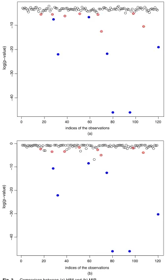
Applying HIM and MIP to these data with the FDR level atα=0:05, HIM finds 15 influen-tial observations, whereas MIP obtains seven influeninfluen-tial observations. Interestingly, the set of influential points by MIP is a subset of that by HIM. In Fig. 3, we plot the influential obser-vations that were found by MIP as full circles and the extra influential obserobser-vations by HIM as crossed circles, where they-axis denotes the logarithm of thep-values that were obtained by using HIM as in Fig. 3(a) or using MIP as in Fig. 3(b). To make the plot more comparable, the checking step in the min-max-checking algorithm is applied to all observations such that we can obtain ap-value for each observation. From Fig. 3(b), we can see that the crossed circles that are identified by HIM as influential do not seem to have very smallp-values.
To make further comparison, we use OLS estimation on the important variables found via the lasso, after applying either HIM or MIP, to the non-influential point set that was identified by HIM. We compare their Bayesian information criterion BIC-score defined as BIC=nlog.RSS=n/+klog.n/where RSS is the residual sum of squares,n=105 is the sample size after removing the 15 influential points that were identified by HIM, andkis the number of variables used. Obviously, a model with a smaller BIC is preferred. Note thatk=9 if HIM is used andk=6 if MIP is applied. Because of the set-up, this comparison favours HIM in some sense. It is found that BIC= −567:34 if HIM is applied for influential point detection and BIC= −578:94 if MIP is applied. Thus, MIP is potentially more effective for finding a better model than HIM as its BIC-value is smaller.
For the real data, of course it is not known which observations are influential. To assess the performance of HIM and MIP further, we artificially add influential points to the data set and evaluate whether they can find these points afterwards. Specifically, we first remove the influential points that were detected by each method and add 10 additional observations to the remaining data. This scheme gives a total of 115 observations for assessing HIM and 123 observations for MIP. The 10 added influential observations are generated asXiS=1:1xS+ZS,XiSc=xSc,Yi= 1:1y+, 1i10, whereZ∼N.0, 0:01Ip/,Sis a random subset of{1,: : :,p}consisting of 10 distinctive indices,ZS is a subvector ofZwith indices inS,.x,y/is chosen randomly from a non-influential point set identified by HIM and∼N.0, 0:01/is independent ofZ.
We apply MIP and HIM to the contaminated data defined above with the nominal FPR set as 0:05 in the Benjamni–Hochberg procedure and repeat the process 100 times. Then we compute the TPR and FPR of the two methods for identifying these artificial influential points. It turns out that MIP gives a TPR of 1 and an FPR of 0.008, whereas HIM gives a TPR of 1 and an FPR as high as 0:585. Obviously, HIM suffers seriously from the swamping effect that is caused by the addition of new influential observations, wheres MIP does not seem to be affected by newly added observations.
5.2. Low dimensional data sets
We now apply MIP to two classical data sets with small p that are used extensively in the literature as benchmark cases for influential diagnosis.
indices of the observations
log(p−v
a
l
u
e)
0 20 40 60 80 100 120
−40
−
3
0
−
20
−10
0 20 40 60 80 100 120
−40
−
3
0−
2
0
−
1
0
0
indices of the observations
log(p−v
a
l
u
e)
(a)
[image:21.485.78.413.55.623.2](b)
can see that the TPR of MIP is 0.6, whereas its FPR is 0. However, if we examine just Cook’s distance by using leave-one-out observation, the TPR becomes 0 and the FPR becomes 0.0625. If the DFFITS-statistic is used for identifying outliers, then the TPR is 0 and the FPR is also 0. Neither Cook’s distance nor DFFITS has any power in detecting these outliers.
For the second case, we look at a data set withp=3 that is designed to have masking and swamping effects (Hawkinset al., 1984; Nurunnabiet al., 2014). There aren=75 observations in total, the first 10 of which are specifically perturbed to be influential. Interestingly, after applying MIP, we find the first 13 observations as influential, meaning that the TPR of MIP is 1 and its FPR is 0.046. If we apply Cook’s distance only, the TPR becomes 0 and the FPR is 0.0615, whereas the TPR becomes 0 and the FPR becomes 0 if we apply the DFFITS-statistic for outlier detection. For this example, MIP is much more powerful with a controlled FDR.
We point out that, to use MIP, we require min{n,p}→ ∞, though the rates of n andp going to∞ can be arbitrarily slow. From the analysis of the two low dimensional data sets above, however, we can see that MIP continues to provide useful results and at least is more competitive than examining Cook’s distance or the DFFITS-statistic naively.
6. Discussion
We have proposed a novel procedure named MIP for multiple influential point detection in high dimensional spaces. The MIP procedure is intuitive, theoretically justified and easy to implement. In particular, by combining the strengths of the max- and min-statistics, the MIP framework proposed can overcome the masking and swamping effects that are notorious in influence diagnosis, and it can identify multiple influential points with prespecified accuracy in terms of FDR control which is empirically verified by extensive simulation.
Both HIM and MIP are based on the idea of measuring the change in marginal correlations when one observation is removed. The primary consideration for using the marginal correlation is due to its ubiquity in statistical analysis and the possibility of deriving rigorous theoretical results, as we have shown. But it need not be the only quantity that defines influence. Towards this, it will be interesting to explore the use of other quantities to define influence. In this paper, we have confined our attention to linear regression. An interesting topic for future research is to extend the idea to other models such as the generalized linear model. A major challenge, however, is to define a tractable influence measure that is similar to HIM.
Finally, we hope that this paper brings to the attention of the statistics community the im-portance of influence diagnosis and how one might think about defining influence and devising automatic procedures for assessing influence, in a theoretically justified fashion. With the rapid advances in ‘big data’ analytics, we believe that the issue of influence diagnosis will only become more relevant and we hope that this paper can serve as a catalyst to stimulate more research in this area.
Acknowledgements
We thank three reviewers, the Associate Editor and Joint Editor for their helpful comments that have led to a much improved paper.
References
Aggarwal, C. C. and Yu, P. S. (2001) Outlier detection for high dimensional data.ACM Sigmod Rec.,30, 37–46. Belsley, D. A., Kuh, E. and Welsch, R. E. (1980)Regression Diagnostics: Identifying Influential Data and Sources
of Collinearity. New York: Wiley.
Benjamini, Y. and Hochberg, Y. (1995) Controlling the false discovery rate: a practical and powerful approach to multiple testing.J. R. Statist. Soc.B,57, 289–300.
Billor, N., Hadi, A. S. and Velleman, P. F. (2000) Bacon: blocked adaptive computationally efficient outlier nominators.Computnl Statist. Data Anal.,34, 279–298.
Brownlee, K. A. (1965)Statistical Theory and Methodology in Science and Engineering. New York: Wiley. Chatterjee, S. and Hadi, A. S. (1986) Influential observations, high leverage points, and outliers in linear regression.
Statist. Sci.,1, 415–416.
Chiang, A. P., Beck, J. S., Yen, H. J., Tayeh, M. K., Scheetz, T. E., Swiderski, R. E., Nishimura, D. Y., Braun, T. A., Kim, K. Y., Huang, J., Elbedour, K., Carmi, R., Slusarski, D. C., Casavant, T. L., Stone, E. M. and Sheffield, V. C. (2006) Homozygosity mapping with SNP arrays identifies trim32, an e3 ubiquitin ligase, as a Bardet-Biedl syndrome gene (bbs11).Proc. Natn. Acad. Sci. USA,103, 6287–6292.
Cook, R. D. (1977) Detection of influential observation in linear regression.Technometrics,19, 15–18. Draper, N. R. and Smith, H. (2014)Applied Regression Analysis, 3rd edn. New York: Wiley.
Fan, J., Fan, Y. and Barut, E. (2014) Adaptive robust variable selection.Ann. Statist.,42, 324–351.
Fan, J. and Lv, J. (2008) Sure independence screening for ultrahigh dimensional feature space (with discussion).
J. R. Statist. Soc.B,70, 849–911.
Filzmoser, P., Maronna, R. A. and Werner, M. (2008) Outlier identification in high dimensions.Computnl Statist.
Data Anal.,52, 1694–1711.
Friedman, J., Hastie, T. and Tibshirani, R. (2010) Regularization for generalized linear models via coordinate descent.J. Statist. Softwr.,33, 1–22.
Hadi, A. S. and Simonoff, J. S. (1993) Procedures for the identification of multiple outliers in linear models.
J. Am. Statist. Ass.,88, 1264–1272.
Hawkins, D. M., Dan, B. and Kass, G. V. (1984) Location of several outliers in multiple-regression data using elemental sets.Technometrics,26, 197–208.
Huang, J., Ma, S. and Zhang, C. H. (2006) Adaptive lasso for sparse high-dimensional regression.Statist. Sin.,
18, 1603–1618.
Huber, P. J. and Ronchetti, E. M. (2009)Robust Statistics, 2nd edn. New York: Springer.
Imon, A. H. M. R. (2005) Identifying multiple influential observations in linear regression.J. Appl. Statist.,32, 929–946.
Lawrance, A. J. (1995) Deletion influence and masking in regression.J. R. Statist. Soc.B,57, 181–189. Maronna, R. A. (2011) Robust ridge regression for high-dimensional data.Technometrics,53, 44–53.
Maronna, R. A., Martin, R. D. and Yohai, V. J. (2006)Robust Statistics: Theory and Methods. New York: Wiley. Nurunnabi, A. A. M. (2011) A diagnostic measure for influential observations in linear regression.Communs
Statist. Theory Meth.,40, 1169–1183.
Nurunnabi, A. A. M., Hadi, A. S. and Imon, A. H. M. R. (2014) Procedures for the identification of multiple influential observations in linear regression.J. Appl. Statist.,41, 1315–1331.
Pan, J., Fung, W. and Fang, K. (2000) Multiple outlier detection in multivariate data using projection pursuit techniques.J. Statist. Planng Inf.,83, 153–167.
Ro, K., Zou, C., Wang, Z. and Yin, G. (2015) Outlier detection for high-dimensional data.Biometrika,102, 589–599.
Roberts, S., Martin, M. A. and Zheng, L. (2015) An adaptive, automatic multiple-case deletion technique for detecting influence in regression.Technometrics,57, 408–417.
Rousseeuw, P. and Hubert, M. (2011) Robust statistics for outlier detection.Data Minng Knowl. Discov., 1, 73–79.
Rousseeuw, P. J. and Leroy, A. M. (1987)Robust Regression and Outlier Detection. New York: Wiley.
Rousseeuw, P. J. and van Zomeren, B. C. (1990) Unmasking multivariate outliers and leverage points.J. Am.
Statist. Ass.,85, 633–639.
Satopaa, V., Albrecht, J. R., Irwin, D. E. and Raghavan, B. (2011) Finding a kneedle in a haystack: detecting knee points in system behavior. InProc. Int. Conf. Distributed Computing Systems, Minneapolis, pp. 166–171. New York: Institute of Electrical and Electronics Engineers.
She, Y. and Owen, A. B. (2011) Outlier detection using nonconvex penalized regression.J. Am. Statist. Ass.,106, 626–639.
Shieh, A. D. and Hung, Y. S. (2009) Detecting outlier samples in microarray data.Statist. Appl. Genet. Molec.
Biol.,8, 1–24.
Smucler, E. and Yohai, V. J. (2017) Robust and sparse estimators for linear regression models.Computnl Statist.
Data Anal.,111, 116–130.
Tibshirani, R. (1996) Regression shrinkage and selection via the lasso.J. R. Statist. Soc.B,58, 267–288. Velleman, P. F. and Welsch, R. E. (1981) Efficient computing of regression diagnostics. Am. Statistn, 35,