Theoretical chemistry

A thesis

submitted in partial fulfilment

of the requirements for the Degree

of

Doctor of Philosophy in Chemistry

in

the

University of Canterbmy

by

Pravit Sudkeaw

University of Canterbury

Contents

Chapter 1 Theories and Computational Methods

Introduction 1

1.1 Schroedinger Equation 2

1.2 Molecular Orbital Theory 5

1.3 Basis Set 6

1.4 The Variation Method and Hartree-Fock Theory 9

1.5 Closed-shell Systems 10

1.6 Open-shell Systems 12

1.7 Configuration Interaction 14

1.8 M~ller-Plesset Perturbation Theory 15

1.9 GAUSSIAN Program 18

1.10 MICROMOL Program 25

1.11 The Valence-Bond method 25

1.12 The Valence-Bond Program 27

1.13 SemiempiricalMethods 28

1.13.1 Complete Neglect of Differential Overlap

(CNDO) 29

1.13.2 Complete Neglect of Differential Overlap,

Version 2 (CND0/2) 31

1.13.3 Intermediate Neglect of Differential Overlap

(INDO) 32

1.13.4 Neglect of Diatomic Differential Overlap

(NDDO) 33

1.13.5 Modified Intermediate Neglect of Differential

Overlap (MINDO) 34

1.13.6 Modified Neglect of Diatomic Overlap

1.13.8 Parametric Method Number 3 (MNDO-PM3) 37 Chapter 2 The Proton Affinity Study of Diacetylene

2.1 Introduction 39

2.2 Theory 39

2.3 Method of Calculation 41

2.4 Results 42

2.5 Discussion 47

2.6 Conclusion 49

Chapter 3 Ab Initio Study of the Reaction between CH3CN and CH3+

3.1 Introduction 50

3.2 Method of Calculation 51

3.3 Results and Discussion 60

3.4 Conclusion 64

Chapter 4 Ab Initio Study of Organotin Compounds

4.1 Introduction 65

4.2 Method 65

4.3 Results 67

4.4 Discussion 77

Chapter 5 Theoretical Study of CnO, CnO+, CnHO+, CnS, CnS+ and CnHS+ Species

5.1 Introduction 79

5.2 Computational Details 84

5.3 Results and Discussion 84

5.3.1 Optimized Geometries 85

5.3.2 Rotational Constants 89

5.3.3 Dipole Moments 90

5.3.6

5. 3. 7 Harmonic Vibrational Frequencies

5.

5.4

Chapter

6

6.1

6.2

6.3

6.4

Chapter 7 Valence-Bond Study of the BH2 Radical

7.1

7.2 Method of Calculation

7.3

7.4

Acknowledgements References

Appendix Physical Constants and Conversion Factors Glossary of symbols

93

94 95

97

104

111

143

page

1.1

38

2.1

degrees)

43

2.2

44

2.3

correction (kJ moi-l)

44

2.4

45

2.5

46

3.1

of theories and basis sets

52

3.2

vibrational energies of molecules with the

4-31G

55

3.3

58

3.4

possible intermediates, relative to CH3CNCH3+

59

4.1

Hartree-Fock level with the

3-21G*

69

4.2

zero-point vibrational energies (kJ mol-l) for organotin compounds

70

4.3

Hartree-Fock level with the

3-21G*

72

4.4

this study with other works

73

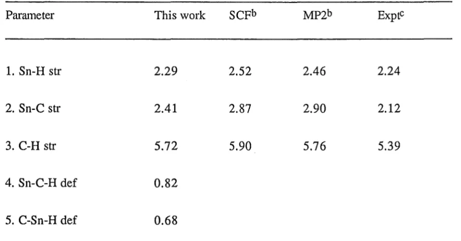
4.5

results and other works

73

4.6

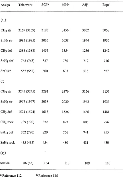
4.7 Calculated energies of stannane (hartree) as obtained by different methods 74 4.8 Comparison of geometries of methyl stannane (Angstroms and degrees)

with other works 75

4.9 Compadson of force constants found for methyl stannane 75 4.10 The calculated hat.monic vibrational frequencies ( cm-1) for

methyl stannane 76

5.1 Optimized geometries (Angstroms and degrees) of oxygen and sulphur containing species (grouped in pairs for compadson) 88 5.2 Calculated rotational constants of CnO, CnO+, CnS and CnS+,

comparing with available expedmental values 89

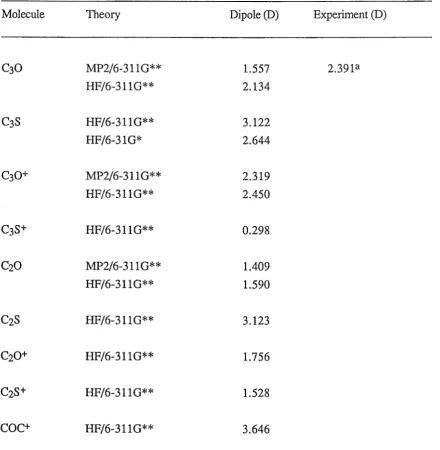
5.3 Calculated dipole moments of CnO, CnO+, CnS, CnS+ and COC+

in Debye (D) 90

5.4 Calculated adiabatic ionization energies for C30, C3S, CzO and CzS at

the MP4SDQ level of theory and a 6-3110** basis set 91 5.5 Calculated proton affinities for C30, C3S, CzO and CzS at the MP4SDQ

level of theory with 6-310* and 6-3110** basis sets 92 5.6 Calculated dissociation energies at different levels of theory and

experimental values for C30, C3S, CzO and CzS 93

5.7 Calculated harmonic vibrational frequencies (cm-1) at different levels

of theory and experimental values for C30, C3S, CzO and CzS 94 5.8 Calculated heat of formation for C30, C3S, CzO and CzS at the

MP4/6-3110** level of theory compm·e with other's works 96 5.9 Energies of CnO, CnO+, HmCnO+, CnS, CnS+ and HmCnS+ species at

different levels of theory and basis sets 98

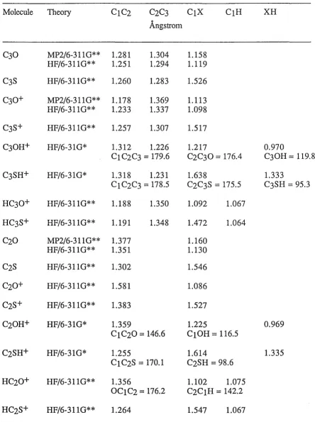
5.10 Optimized geometric parameters for CnO, CnO+ and CnHO+ species in

Angstroms and degrees 99

5.11 Optimized geometdc for CnS, CnS+ and CnHS+ species at different levels

of theory in Angstroms and degrees 100

unsealed zero-point vibrational energies 103 5.14 Proton affinities of CnO and CnS species calculated including

unsealed zero-point vibrational energies 103

6.1 GAUSSIAN 82 calculated energies of compounds (hartree) with

4-31G and 6-31G* basis sets 130

6.2 Calculated ha1monic vibrational frequencies (cm-1) and zero-point

vibrational energies of molecules (kJ mol-l) with a 4-31G basis set 131

6.3 The relative energies (zero-point vibrational energy corrected) between

reactants, C2H2 and C4H2+ and C6H4+ isomers 134

6.4 Heat of formation and zero-point vibrational energies of molecules by

the AM1 method 135

6.5 The AM1 calculated ha1monic vibrational frequencies (cm·l) for

C6H4 + isomers 136

6.6 The AM1 calculated relative energies between C2H2 + C4H2+ and

C6R4+ isomers (kJ mol-l) 141

6.7 Order of relative energies (kJ mol-l) for C6H4+ isomers with

C2H2 + C4H2+, compared between the AM1 and the Haiiree-Fock method 142 6.8 Optimized geometries of C4H2+ (Angstroms) from AM1, HF/6-31G*

and an experiment 142

6.9 Comparison of the heats of formation for isomers of C6R4+ from

the AM1 method with experiment 143

7.1 Exponent and coefficient values of best orbital energy basis set

7.4

1.238

HBH =

129.9

150

7.5

151

7.6

energies (hartree)

152

page

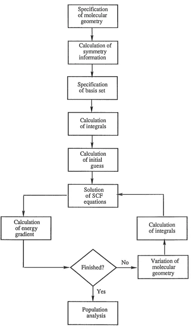
1.1 Flow diagram for the SCF calculation 19

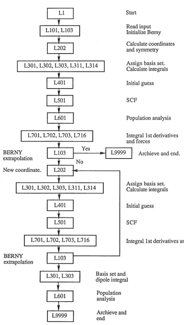
1.2 Sequence of Links in a Hartree-Fock Optimization 24

1.3 Flow diagram for the Valence-Bond program 28

2.1 6-310* optimized structures of C4H2 and C4H3+ 41

2.2 The change in electron population on each atom after an addition

of a proton to a terminal of C4H2 48

2.3 The change of HOMO of C4H2 after protonation process 49 3.1 Optimized structures of compounds with 6-310* basis set

(Angstroms and degrees) 53

3.2 Energy diagram (kJ mol-l) for C3H6N+ isomers from this study

(with scheme 1) 61

3.3 Energy diagram (kJ mol-l) for C3H6N+ suggested by ref. [145]

(with scheme 2) 63

4.1 Optimized structures of organotin compounds (Angstroms and degrees) 68 5.1 Structures found for CnO, CnO+, CnHO+, CnS, CnS+ and CnHS+ species 87

6.1 Structures of molecules in AM1 calculations 108

6.2 Main chemical process of the reation between CzHz and C4H2+ 111

6.3 1-3 sigmatrotopic proton shift in isomer (7) 112

6.4 1-2 proton shift in isomer (7) 113

6.5 Energy diagram for the pathway A 114

6.6 Energy diagram for the pathway B 114

6.7 The formations of cyclic isomers 115

6.8 Dissociative pathway for 5-membered ring isomer 116 6.9 Rearrangement process for propene structure isomer 116 6.10 Rearrangement process for benzyne structure isomer 117

6.13 Optimized structures from the AMI method (Angst:t·oms and degrees) 6.14 Optimized structures (Angstroms and degrees) from the Hartree-Fock

method, (1) to (7) using a 6-310* basis set and (8) to (12) using a 4-310 basis set

120

Ab initio Molecular Orbital and Valence-Bond methods and the semiempidcal, AMl

method are applied in the studies of:

1. The proton affmity of diacetylene

The gas-phase ion-molecule reaction between diacetylene and a proton was studied theoretically at the MP4SDQ/6-311G** level. The geometries, calculated harmonic

vibrational frequencies and the proton affmity of the most stable structures ar·e repmied. The results from this study are supported by selected ion flow tube measurements and ar·e

compared with other calculations

2. The gas-phase reaction of CH3CN and CH3+

The reaction between CH3CN and CH3+ was studied at the MP4SDQ/6-31G* level of theory in order to determine the products and establish the multistep dissociation pathway of the reaction. The location and height of the transition states in the process is used as a critetia for the feasibility of the proposed pathway. The result is compared with the expedmental and theoretical studies of the same system done by Wincel and coworkers [146].

3. The geometdes and force constants of small-sized organotin compounds The calculations on 12 small-sized organotin compounds were done at the

HF/3-210* level of theory. The objective of this study was to provide the force constants of Sn-X andSn-X-Sn-Y types for the use in Molecular Mechanic calculations of organotin

compounds. The calculated geometries and hrumonic vibrational frequencies of stannane and methyl stannane are compru·ed with expedmental results in order to measure the

reliability of the calculations.

4. The chemical properties of CnO, CnO+, CnHO+, CnS, CnS+ and CnHS+ species in the instellar clouds

MP4SDQ/6-311G** level of theory. The calculations suggest that these species are more stable in protonated forms and could be intermediates of some steady state processes.

5. Theoretical study of C6H4+ formation in acetylenic flames

~H4+ has been detected as an intermediate in acetylenic flames. The semiempirical AMl method was used to determine the most stable products and to establish a chemical mechanism of the reaction between C4H2+ and C2H2. The results from AMl method were refined by ab initio calculations at the HF/4-310 andMP4SDQ/6-31G* level. From this study, only chemical pathways involved acyclic structure isomers are feasible.

6. A Valence-Bond study of BH2 radical

In this study a Valence-Bond program was used on IBM PC/ AT microcomputer to study the correlation between the nuclear bond angle and the angle of hybrid orbitals of BH2. The energies ofBH2 from the Valence-Bond calculations were also compared with the energies from the Molecular Orbital method at the HF, MP4SDQ and CI level with best orbital energy basis sets, 10s6p/2slp for boron atom and 6s/ls for hydrogen atoms.

Theories and Computational Methods

Introduction

Mter nearly eighty years of development, quantum chemistry has come to play an important part in the study of chemical structures and molecular properties. The subject now has become more mature and the study of medium-sized molecules in gaseous phase is practical. Various kinds of calculation are available and can be used by a non-theorist as a guide or a complement to his experiments. Though many theories in quantum chemistry have become more and more complicated, their implementation on digital computers has allowed any chemist with a general background in quantum chemistry and some computer experience to use the calculations.

The two main theories in quantum chemistry are the Molecular Orbital theory (MO) and the Valence-Bond theory (VB). The MO theory is based on the rather physics-type point of view of free electrons moving in a potential field of fixed nuclei whereas the VB theory comes from the chemical bonding idea in which electrons from adjacent atoms use their electrons to build the chemical bonds in forming molecules. Though the VB theory has a longer history and gives better pictures of chemical bonds than the MO theory, most of molecular calculations in the past 30 years use MO theory. This stems from the difficulties

in the numerical mathematics and in the finding of a complete set of electron configurations for the input which is required in the VB calculation.

Calculations in quantum chemistry are divided into ab initio methods and

semiempirical methods. Ab initio methods require only the structure, geometry and basis functions for the starting parameters. The calculations then follow the relevant theory. In the semiempirical method, some required values such as one-electron integrals are deduced

This thesis is concemed with the application of both MO and VB theory. All calculation were done at the ab initio level except topic 5 in which semiempirical AM1 method was employed after convergence difficulties occurred.

The topics are:

1. The proton affinity of diacetylene. 2. The reaction of CH3CN and CH3+.

3. The theoretical study of chemical properties of small-sized organotin compounds.

4. The chemical properties of CnO, CnO+, CnHO+, CnS, Cns+ and CnHS+ species in the interstellar clouds.

5. Theoretical study of C6H4+ formation in acetylenic flame. 6 Valence Bond study of the BH2 radical on an IBM PC.

Projects 1-5 used the GAUSSIAN 82 and GAUSSIAN 90 program [11,53]. Only the project 5, MOPAC version 6.0 [135] was used.

The work on BH2 used the Micromol Mark III program [28] and a VB program written originally by Maclagan [88].

In this chapter the background and the methods in quantum chemistry that were

used in this thesis are discussed only in a broad manner. The full details are avoided because there are many excellent references [26,62,81].

Though the GAUSSIAN program series is well-known, a brief description of its features is given, together with the other two programs.

1.1 Schroedinger Equation

All molecular orbital calculations are approximate solutions of the Schroedinger equation [126]. The equation has its origin in the de Broglie equation:

h

p=-A, (1.1)

E=hV (1.2)

The frequency of radiation v is related to the wavelength by the relation:

c

where c is the velocity of light.

The Schroedinger equation for a stationary state is the combination of the de Broglie relation and the classical differential equation of a simple harmonic three-dimensional

standing wave. The general f01m of the equation is:

H'¥

=

The Hamiltonian operator, H is defined as

H=T+V (1.5)

The kinetic energy operator, T, is a sum of differential operators,

(1.6)

The sum is over all particles i, which here are electrons and nuclei, and mi is the mass of each particle.

The potential energy operator, Vis the coulomb interaction operator,

(1.7)

The sum is over distinct pairs of particles (i,j) with electric charges ei and ej- The parameter fij is the distance between the two particles. The Hamiltonian in this equation is classified as a non-relativistic one.

The Schroedinger equation for any molecule will have many solutions, corresponding to different stationary states. The ground state is the state with lowest

Born-Oppenheimer approximation [14] is used to simplify the Schroedinger equation as

H elec lpelec(r,R) = Eeff(R) lpelec(r,R) (1.8)

which corresponds to the motion of electrons in the field of fixed nuclei.

'Jidec is the electronic wavefunction and the Hamiltonian, Helec, is defmed as H elec = T elec

+

v

where T elec is the electronic kinetic energy,

(

2 2 2

J

(

h2

J

Telec=-

L

+ +

-8_1t 2 _{l11e 1} . _axi 2 _{ay i} 2 _a~ 2

and V is the coulomb potential energy, electrons nuclei

G

V=-

I

I

i s ris 1 < j (

e2) nuclei

--:: +

I I

riJ s < t

(1.9)

(1.10)

(1.11)

In practice, the units of parameter in the Schroedinger equation are changed to atomic unit which makes the equation take a more simple form.

The Bohr radius is defined unit of length as

and new coordinates (x', y', z') are written as the,

I X

X = -ao

In similar way, a new unit of energy, the hartree, is defined as

e2

EH= =27.2114eV. 41tfQao

The new energy is given by

El -

_g_

-EH

The Schroedinger equation in atomic units is H' '¥'

=

where the Hamiltonian, H', in the atomic unit, is

(1.12)

(1.13)

(1.14)

(1.15)

(

2 i

a

a

a

xi Yi zi

electrons nuclei(Zs) electrons

-

2:

2: -..

2: 2:

i s r ts i < j

1.2 Molecular Orbital Theory

(

1 ) nuclei

T-

2: 2:

IJ S

<

(1.17)

In the Molecular Orbital theory, the full wavefunction is approximated by products of one-electron functions (or orbitals). A Cartesian coordinate function for a single electron is assigned as 'l'(x,y,z). The spin coordinate,~. is included in each molecular orbital to give

1 d ' . E h . f ' h . 1 1 1 · . f

a comp ete escnpt10n. ac spm unct10n can ave two spm va ues

+2

-2

1 a(+

2)

1

P<+2)

= o

1

a(-

2)

=

1

P<-2)

The combination of a spin function and a Cartesian coordinate function gives a spin orbital, X(x, y, z, ~).

The spin orbitals of n electrons are combined in a determinant which is a wavefunction of the system and also has the required antisymmetric property.

'¥determinant= (n!)-l/2

XI(l) X20)

X1(2) X2(2)

Xn(1) Xn(2)

XI (n) Xz(n) Xn(n)

(1.19)

The orthonormal molecular orbitals have the properties:

and

(1.20)

A full wavefunction for a closed-shell molecule with n (even) electrons, doubly occupying

~

'l'l(l)a(1) '1'1(1)~(1) '1'2(1)a(1) 'lft(2)a(2) '1'1(2)~(2) 'l'2(2)a(2)

'Vl

'Vn/2(1)~(1) 'Vn/2(2)~(2)

(1.21)

This determinant is always referred to as a Slater determinant. (n!)-1/2 is the nonnalizing factor which is added to ensure that,

(1.22)

1.3 Basis set

The basis set is a set of functions such that each one is used to represent one electron orbital. A molecular orbital can be built from the basis set,~~. ~2. ~3 ... ~n. as

N

'Vi=

L

CJ.ti~i

J.L=1

where CJ.ti are molecular orbital expansion coefficients.

(1.23)

STOs are mostly used for the calculations of wavefunction for atoms or small molecules. They are found to be not suitable for usual molecular calculations because of numerical difficulties. The functions in STOs are labeled like hydrogen atomic orbitals, ls, 2s, 2px ... and have a normalized form,

(

~~

J

~2r)

=

961t r exp

2

(

~~

J

(-~2r)

=

321t x exp

2

(1.24)

where ~i are constants called the orbital exponents.

The GTFs functions are powers of x, y and z multiplied by exp(-ar2). The constant, a, determines the size of the functions. The first ten normalized GTFs functions

are

3/4

g,(

a,

=

L"")

1/4

gx(O<, r)

=

c~JaS)

(

128a5) 114 gy(a, r) = 1t

3 y exp (-ar2)

(

128a5) 114

gz( a, r)

=

1/4 (

2048ct7) gyy(ct, r) =

9

Jt

3 y2 exp (-crr2)

1/4

(

2048ct7) gzz(ct, r) =

91t3 z2 exp (-ctr2) 1/4

(

2048ct7) gxy( ct, r) = Jt

3 xy exp ( -crr2)

1/4

(

2048ct7) gxz(ct, r) = Jt

3 xz exp (-crr2)

1/4

(

2048ct7) gyz( ct, r) = Jt

3 yz exp ( -m2)

(1.25)

GTFs functions cannot fully represent atomic orbitals because they do not have a cusp at the origin. It needs a linear combination of several GTFs functions (so-called 'primitive gaussian') to give more suitable basis functions, which are termed as 'contracted gaussians'. An s-type basis function $J..l can be expanded in terms of s-type GTFs as:

(1.26)

where the coefficients, dJ..lS, are fixed.

The three types of basis set that were used in this thesis are:

1. A contracted basis sets 10s6p/2slp for boron atom and 6s/ls for hydrogen atom were used in the VB calculation of BH2 molecule. This basis set was taken from Poirier et al. [104] and F.B.v. Duijneveldt [46]. The basis set consists of

best-energy -orbital atomic orbitals in term of K primitive gaussian functions: K

$nl(~=l, r) =

L

k=l , ' (1.27)

standard basis sets and used in the calculations on GAUSSIAN 82. Functions in this basis sets are separated into two groups, inner shells and valence shells. Each inner shell is represented by a single function which is composes of K primitive gaussian functions. The general expression for an inner shell function is:

K

$nt(r) =

2:

(1.28)

where K = 3, 4, and 6 for the basis sets, 3-21G, 4-31G and 6-31G. The subscripts, n and l are used to specify atomic functions, for example,

$2s·

The valence shell is represented by two functions which are expanded in K' and K" gaussian primitives. The general expression for these functions are:

K'

~nlr)

=

2:

k=1 • ' (1.29)

and

K"

Mhir) =

2:

'I' k=1 • . (1.30)

where K'=2 and K"=1 in the basis set 3-21G, and so forth.

3. Polarization basis sets 6-31G* and 6-31G**· These basis sets are split-valence type including polarization function which are also provided in GAUSSIAN 82 as standard basis sets. In 6-31G* basis set, a set of polarization functions, of higher angular momentum quantum number (d-type for the ftrst-row heavy atoms, not hydrogen) are added to the split-valence 31G basis set. When p-type functions are added to hydrogen in the polarization 6-31G* basis set, it becomes more complete basis set and is termed 6-31G**.

1.4 The Variation method and Hartree-Fock theory

quantum mechanics [82]. An expectation value of energy corresponding to <I> which is any

antisymmetric normalized function of the electronic co-ordinate, can be written as:

E' =

J

If <I> is the exact wavefunction, 'I', for the electronic ground state, the energy will be

E'

=

J'P*

=

In the case that <I> is any other normalized antisymmetric function, it can be shown that

E' = J<I>*H <I> dt > E (1.33)

In the variation method, the expansion coefficients, Clli• are adjusted until the lowest value of energy, E', is obtained. This energy will be the closest upper bound to the exact energy within the limitation of the single-determinant wavefunction and the chosen basis set. With this process, it will give the optimum orbitals and the best single-determinant wavefunction, in the energy sense. The variational equation is

aE'

- = 0

OCJ.!i for all ~ and i

1.5 Closed-shell Systems

A consequence of applying the variational condition to the closed-shell wavefunctions (1.21) is the Roothann-Hall equations [60,118]:

N

L(FJ.!v - eiSJ.!v)Cvi

=

V=1

with the orthonormality conditions:

N N

*

2: 2:

s

=

~=

1

Jl

= 1, 2, ... N

(1.34)

(1.35)

S11v are the elements of an N by N overlap matrix:

(1.37)

F11v are the elements of the N X N Pock matrix:

core N N 1

F = H

+

:L :L

2

(1.38)

Hcore is the matdx of the single electron energy in a field of 'bare' nuclei. It is

llV

defmedas:

where

core

J

H

=

llV (1.39)

(1.40)

ZAiS the atomic number of atom A and M is a number of atoms in a molecule. The terms, (llVIA.cr), are two-electron integrals,

(1.41) The density matrix, PA.cr, is defined as:

ace

*

P,.. =2

L

1\,cr i=1 1\,l m (1.42)

The fmal formula for the molecular electronic energy, Eee, is

ee 1 N N core

E

=

2

:L :L

+

!l=1V=1 llV !lY llV

The electronic energy when added to the nuclear repulsion energy, Enr, will give the total energy of the molecule.

MM

E

=

L L

nr A< B RAB (1.44)

An iterative process is needed to solve the Roothaan-Hall equation because the Pock-matrix depends on the molecular orbital coefficients, c~, which are also the solutions of the equation. A set of coefficients is first guessed or calculated by a semiempirical method. These values are used as the beginning of a calculation which will generate a new set of coefficients and the energy of the system. The new wavefunction is used for the next iteration until there is no change in either energy value or the density matrix. This give the term 'self-consistent field (SCF) ' to the method.

The full single determinantal wavefunction from the Hartree-Fock method will be improved by using a more complete basis set. This makes the calculated energy lower, approaching the Hartree-Fock limit which lies above the true energy. The limit cannot reach the true energy because a single determinantal wavefunction fails to describe the conelated motion of the electrons and the exchange term in Hartree-Fock Hamiltonian can only be descdbed in terms of conelation. The energy difference between the Hartree-Fock limit and the true energy is termed the conelation energy.

To do a calculation beyond the Hartree-Fock limit, more Slater determinants of

other electron configurations must be included in a wavefunction. Configuration Interaction (CI) and M~ller-Plesset (MP) [97] are two main methods that are used to obtained multiple

determinant wavefunction.

1.6 Open-Shell systems

An open-shell molecule is a molecule that has unpaired electrons, for example, a

method, a single set of molecular orbitals is used. Some of the molecular orbitals are doubly-occupied and some are singly-occupied. The electrons in these two sets of

molecular orbitals are treated differently in the calculations but the optimization of the system is still based on the variation condition (1.34).

In the UHF method, two different sets of molecular orbitals,

'!'?'and

'I'P,

and~

N a

'!'?' =

I

This leads to the UHF generalization of the Roothaan-Hall equation:

N

a

a

I

=

~ (F~

cPs )

c~.

=

V=1 JlV 1 JlV V1

i

=

Jl

=

The Pock matrices are now defined by

a

a

F = H

+

I

I

+

~ ~ ~1~1 cr

~ core N N a ~ ~

F = H +

I

I

JlV JlV _{A-= 1 cr=1} ~~.cr ~~.cr ~~.cr

The density matrices,

P~cr

P~cr

a aocc a* a

P =

I

A.cr i=1 A.i oi'

~

~occ ~* ~

P

=

I

A.cr i=1 A-1 m

(1.45) .

(1.46)

(1.47)

The integrals S , H and (~-tvlA.cr) are defined the same as in the Roothaan-Hall l-tV l-tV

equations for the closed-shell systems.

1.7 Configuration Interaction

If a system of n electrons is described by a basis set of N functions, there will be N each of

a

'Po

=

Xl,

xz ... ,

subscripts a, b, c ...

Determinants other than 'Po can be built by replacing one or more occupied spin orbitals, Xi, Xj ... by virtual orbitals, Xa. Xb, .... These new determinants are denoted as 'P8

with s

>

('P~

functions ('Pijb), triple-substitution functions

('Pij~c)

replacement of occupied orbitals by virtual ones.

In the full configuration method, a multiple determinant wavefunction can be written as:

(1.50)

The unknown coefficients, a8, can also be determined by the linear variation method

in the equation:

L

s

where Hst is a configuration matrix element,

The full configuration interaction method is usually not practical because a huge number of determinants, (2N!)/[n!(2N- n)!], are involved. This can be resolved by

truncating the series at a given level of substitution. If only single substitutions are included, it will be referred as 'Configuration Interaction, Singles' or CIS,

occ virt a a 'I' CIS= ao'Po

+

2:

1

a

(1.53)

This will lead to no improvement to the Hartree-Fock wavefunction because there is no interaction between the ground state wavefunction and the singly-excited state

wavefunction due to Brillouin's theorem [19].

The next improvement is Configuration Interaction, Doubles or CID in which only double substitutions are included. The CID wavefunction is,

occ 'I' CID = ao'Po

+

1<

virt ab ab I, I, a .. '£' ..

a< b IJ IJ (1.54)

If both single and double substitutions are included, the model is termed

Configuration Interaction, Singles and Doubles, or CISD. The wavefunction for CISD is: occ

~ ~

1<

virt ab ab I, I, a .. '£' ..

a<b IJ IJ

(1.55)

The calculation process can be reduced further by limiting the number of spin orbitals that are involved. This leads to the terms ' minimum sized window' and 'frozen core approximation' [62].

1.8

Perturbation Theory

elements,

(1.57)

The perturbation, AV, is defined as

AV

=

where H is the correct Hamiltonian.

If A= 0, HA, is the unperturbed Ho but if the A= 1, Ht. will become the correct Hamiltonian, H. The zero-order Hamiltonian, Ho is defined as a sum of the one-electron Pock operators in M~ller-Plesset theory. The value, Es, is a sum of one-electron energies,

Ei, for the spin orbitals which are occupied in a particular determinant 'P s.

According to Rayleigh-Schroedinger perturbation theory [63], the full CI ground state wavefunction and energy of the Hamiltonian Ht. can be expanded in terms of

A

'Pt. = 'P(O)

+ A 'P(l) + A2'P(2) + ...

+ AE(l) + A2E(2)

+ ....

(1.59) (1.60)

The mixing from other configurations into the ground state appears in the perturbation te1ms. The limitation of the mixing is due to the highest order energy term allowed in the calculation and is termed as MP2, MP3, .. MPn. This is different from the limited CI method which directly truncates the matrix involved.

The zero-order terms in (1.55) and (1.56) are,

'P(O) ='Po (1.61)

(1.62)

The M~ller-Plesset energy to first-order is thus the Hartree-Pock energy,

and the contribution to the wavefunction is 'P(l) =

:L

s>O

(1.63)

The contributions of the first-order pe1turbation to the coefficients, as, for the wavefunction,

~(1)

L

as~~O)

s>O

provided that the

~(O)

~(k)'

(1) -1

as =(Eo- Es) Vs0

(1.66)

(1.67)

As in the CI method, the contribution is non-zero only when s corresponds to a double substitution.

The second-order contribution to the M~ller-Plesset energy is D

E(2)

=

s

The E(2) is the summation over all double substitutions. V sO is defined as the

two-electron integral:

Vso = (ijllab) and

(ijllab)

=

fJ

x:

~

) [X a (

l);q,

Ih;,

"2.

The second-order contribution to the energy is

occ

~ ~

1< J

virt -1 2

I, I, (Ea

+

and the third-order contribution to the energy is

D D

E(3) =I, I, (Eo- Es)-1(Eo-Et)-1Vos(Vst- VooOst)Vto

s t

(1.69)

(1.70)

MP4SDQ is the term for the prutial fourth-order perturbation calculation that uses single, double and quadruple substitutions only.

The M$ller-Plesset perturbation method is reliable and effective in most cases but it

should be mentioned that the theory, terminated at any order, is no longer vru·iational. This means that the method can give energies that lower than the true one.

1.9 GAUSSIAN Program

GAUSSIAN 70 developed by the group of J.A. Pople at the Carnegie-Mellon Institute, was introduced in 1970 by Quantum Chemistry Program Exchange (QCPE) as the first ab initio program of the GAUSSIAN series. Though there are many limitations in the program, its speed and simplicity of the input structure made it widely used and it quickly gained acceptance among users. Since then the program has been changed, improved and retitled as: GAUSSIAN 76, GAUSSIAN 80, GAUSSIAN 82, GAUSSIAN 85,

GAUSSIAN 86, GAUSSIAN 88 and GAUSSIAN90. Since most of the work in this thesis was performed on GAUSSIAN 82, the following discussion of the program structure relates mostly to GAUSSIAN 82 [11].

All programs in GAUSSIAN series share the same essential feature of the

calculation processes. The basic input is comprised of three main sections:

1. Geometries written in z-matrix together with charge and spin multiplicity of a

molecule.

2. Basis set specification.

3. The type of calculation with the required level of theory.

The calculation then will start at Hartree-Fock level. Mter the full molecular

wavefunction is obtained, the energy gradients are calculated to fmd the optimized geometry. If the optimization process fails, the calculation process has to go back to the beginning

Calculation of energy gradient

of molecular geometry

Calculation of symmetry information

Specification of basis set

Calculation of integrals

Calculation of initial

guess

Solution ofSCF equations

Finished?

Yes

Population analysis

No

Calculation of integrals

GAUSSIAN 82 was developed from its predecessor, GAUSSIAN 80, by

including more post-SCF procedures, a new package for calculating electrostatic properties and more standard built-in basis sets. The cutoffs for integrals, SCF convergence criteria arid other tolerances were made smaller. This made GAUSSIAN 82 more precise than its predecessor.

GAUSSIAN 82 is made up of 12 overlays in which each one is a group of links. Each link works on a specific task for a part of the whole calculation and has an assigned number for each one. The numbers could be 3 or 4 digits of which the first one or two comprise the overlay number and the last two are the link number. Thus link 301 means that it is link 1 in overlay 3. The overlays in GAUSSIAN 82 are organized as follows:

Overlay 0

The overlay reads the route card then sets up the machine for running the job and defines the sequences of links that are required in the calculation.

Overlay 1

This one is used to set up the geometry and control the optimization procedure. The links in this overlay are

Link 101; reads inputs.

Link 102; controls Fletcher-Powell optimization. Link 103; controls Berny optimization.

Link 104; controls Murtagh-Sargent optimization.

Link 105; calculates force-constant matrix by fmite-difference method.

Overlay2

This overlay converts the z-matrix produced by overlay 1 to standard cartesian coordinates with the center of mass at the origin and assigns the symmetry of the molecule. This is done by the only link in this overlay, Link 202.

Overlay 3

input to the atomic centers.

Link 302; calculates one-electron integrals.

Link 303; calculates dipole integrals.

Link 307; calculates one-electron integral derivatives.

Link 310; primitives two-electron integral program.

Link 311; calculates two-electron integrals for s- and p-orbitals.

Link 312; calculates two-electron integrals for s-, p-, and d-orbitals.

Link 314; calculates two-electron integrals for s-,p-,d-, and f-orbitals.

Link 316; calculates two-electron integral derivatives.

Overlay 4

This overlay contains only one link, link 401.

Link 401; produces an initial guess for the SCF procedure by an INDO or extended

Buckel calculation.

Overlay 5

The overlay contains links that perform different types of SCF calculation.

Link 501; RHF for closed-shell system.

Link 502; UHF for open-shell system.

Link 503; Direct minimization SCF (SCFDM) for RHF and UHF.

Link 505; RHF for open-shell system (ROHF). This link will be used in the case

that link 502 is unreliable because of spin contamination.

Overlatii

This overlay will analyse the wavefunction, produced from the overlay 5.

Link 601; calculates Mulliken population analysis, Fermi contact analysis for the

open-shell system and the dipole moment.

Overlay 7

This overlay is used for the first-, second-derivative force constant calculation.

Link 701; calculates first derivatives of one-electron integrals.

Link 702; calculates first derivatives of two-electron integrals for sp functions. Link 703; calculates first derivatives of two-electron integrals for spd functions. Link 707; calculates second derivatives of one-electron integrals and sum their contribution into the Hartree-Fock force-constants.

Link 708; calculates second derivatives of two-electron integrals and sum their contribution into the Hartree-Fock force-constants.

Link 716; converts cartesian forces and second derivatives to internal coordinates and communicates with optimization control programs.

Overlay 8

This overlay is used for integral transf01mations which are required for post-SCF calculations.

Link 801; setup program for transformation of two-electron integrals, produces molecular orbital coefficient matrix and eigenvalues.

Link 802; transforms integrals for closed- and open-shell using N3 'in-core' algorithm.

Overlay 9

This overlay performs the post-SCF calculations by using the results from overlay

8.

Link 901; forms anti-symmetrized two-electron integrals and computes MP2 energy and first-order MP wavefunction.

Link 902; tests the stability of the Hartree-Fock wavefunction with respect to relaxing of various constraints.

Link 903; is 'in-core' program for closed-shell MP2 calculation. Link 904; is 'in-core' program for open-shell MP2 calculation.

Link 905: is 'in-core' program for closed-shell complex MP2 calculation.

CI calculation.

link 918; produces a new and initial guess for less constrained wavefunction if an instability is detected.

Overlay 10

This overlay is used for calculation of the derivatives of the MP2 and CI energies for optimizations.

Link 1001; calculates the two-electron contribution to the MP2 or CI gradients. Link 1002; produces the derivatives of the MO coefficients from CPHF equation and adds the contribution from CPHF to analytic HF frequencies, CI and MP2 gradients.

Overlay 99

This is the final overlay in any GAUSSIAN 82 job. It produces a summary of the results of the calculation for archiving and reformats ~mays for input to other programs.

Start

Read input Initialize Berny Calculate coordinates and symmetry

L30l,L302,L303,L3ll,L314

L70l,L702,L703,L716

BERNY extrapolation New coordinate.

Initial guess

SCF

Population analysis

Integral 1st derivatives and forces

Archieve and end.

L30l,L302,L303,L3ll,L314

L701,L702,L703,L716

BERNY extrapolation

Initial guess

SCF

Integral 1st derivatives and forces

Basis set and dipole integral

Population analysis

Archieve and end

This program has been developed in the Department of Theoretical Chemistry, University of Cambridge by S.M. Cowell with the assistance from R.D. Amos, N.C. Handy and A.R. Marshall. It was adapted from the Cambridge Analytic Derivative Package (CAD PAC) which itself originated from a version of Dupuis and King's HONDO program [47]. The program was developed on IBM PC/XT and designed to work on

microcomputers with 640Kb of accessible memory.

Micromol Mark III, Micromol Mark V and Micro mol Mark VI are the three

available versions of the program cun·ently. In this work, Micro mol Mark III was used for the calculation of one-electron and two-electron integrals which were required as an input for the Valence Bond program.

The capabilities of Micro mol Mark III are:

1. the evaluation of one-electron and two-electron integrals over contracted cartesian gaussian basis functions of type s, p and d.

2. SCF calculations for closed-shell wavefunctions. 3. calculation of gradients of the energy.

4. use of the gradients for geometry optimization, and for the calculation of force constants by numerical differentiation.

The principal limitations of the program are:

1. a maximum of 63 basis functions. 2. a maximum of 12 shells.

3. a maximum of 12 atoms

4. a maximum of 10 primitive gaussians in any contracted function.

5. a maximum of 110 unique primitives in total.

1.11 The Valence-Bond method

be interpreted as charge-transfer, spin paidng, promotion into a valence state etc. The deformation of wavefunctions mostly involves the electrons in the valence shell which are able to take part in the bonding process, the orbitals in this method are constructed in order to give physical meaning to how atoms interact to form a molecule rather than to be confined in pure mathematical constraint of orthogonality. Thus the VB orbitals are non-orthogonal, which generates some complicated computational problems, particularly in evaluation of the cofactors of determinant formed in evaluating the overlap integrals between wavefunctions. The 'non-orthogonality' problem was resolved when Prosser and Hagstrom [115]

introduced the biorthogonalization technique which directly and efficiently works on non-orthonormal basis orbitals.

In the VB calculation, the eigenvalue equation

(H- ES)C = 0 (1.73)

has to be solved only once. This is different from Molecular-Orbital theory where one has to performed iterations to solve the eigenvalue equation

(F- eS)C

=

The eigenvalues E in the VB calculation correspond to spectroscopic states while theE in MO theory are orbital energies.

Though many efficient matrix methods have been applied to ease the difficulties in the VB method, the MO method is still far more convenient to use and this is the main reason

for the domination of the MO theory in the past three decades. The advantage of the VB method emerges when the electron correlation is considered. In the MO-CI method the full expansion limit can be reached only very rarely and very high cost in computation time and

for a total number of electrons ranging up to about eight. The use of non-orthogonal orbitals in the most accurate wavefunction which is obtained from the truncate CI expansion, petmits a dramatic reduction in the number of terms [27,54,116]. With the advantage of more compact, easily interpretable and accurate wavefunctions, the VB theory has become ·a serious alternative to molecular orbital calculations.

In this study, the VB theory was used to determine the optimized structure of BH2.

1.12 The Valence-Bond program

The package that used in this study originated from Maclagan and Schnuelle's work [88]. It miginally was designed to work on main frame computer and was transferred with small changes to fit in IBM personal computer.

In the calculation process in this program, one-electron and two-electron integrals over atomic basis functions, are the same as those used in the MO method but molecular orbitals are never formed. Instead, all the significant Slater determinant wavefunctions involving atomic orbitals are used to construct the Hamiltonian, H, and overlap, S, matrices. The Hamiltonian operator, H, is defined in atomics units as the equation (1.17):

1 electrons

H=-2

1

electrons nuclei (

z )

-

L

L

+

L L -...

+

L L

i s ris i<j riJ s<t

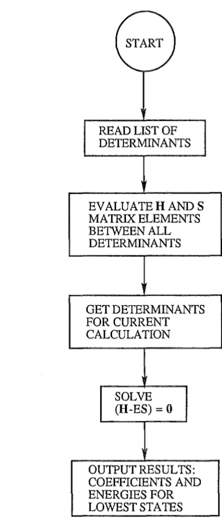
The computational scheme was as follow:

r'fs,Zt)

\ R st

1. Evaluation of one-electron and two-electron integrals. This prut of calculation

was done the program Micromol Mark III which had been described above.

2. Input of details of most important configuration determinants required in the calculation.

3. Evaluation of H and S matrices between all input determinants by using the Presser-Hagstrom biorthogonalization method to evaluate cofactors and then applying Lowdin's formulae [87].

( START )

READ LIST OF DETERMINANTS

EVALUATE HAND S MATRIX ELEMENTS BETWEEN ALL DETERMINANTS

GET DETERMINANTS FOR CURRENT

CALCULATION

SOLVE (H-ES)

=

OUTPUT RESULTS: COEFFICIENTS AND ENERGIES FOR LOWEST STATES

Figure 1.3 Flow diagram for the Valence-Bond program

1.13 Semiempirical methods

:by Dewar [36] to give a more quantitative PMO method. Modem semiempirical methods was initiated when the ab initio methods was found to be impractical for the large polyatomic systems. In the semiempirical approach, the complicated integrals used by ab initio theory were estimated on the basis of empirical data. A mixture of functions based on atomic spectra and on formal theory was used to approximate one- and two-center terms, while three- and four-center integrals were ignored. At present time, the parameters of the semiempirical method which were fmmerly based on atomic spectral data and ab initio results are usually replaced by parameters based on molecular data, to give better

performance. The various levels of semiempirical molecular orbital theory are as follows:

1.13.1 Complete Neglect of Differential Overlap (CNDO)

The CNDO method is the first widely used semiempirical self consistent field method [106,107]. It ignores most of the integrals used in ab initio calculations and approximates the energy in terms of some simple parameters and the retained integrals. Many of the quantities used in this method, such as the two-electron one-center integrals, are

derived from experimental data. The approximations of the CNDO method are:

1. All overlap integrals involving different atomic orbitals are set to zero. The

secular equation:

IF-ESI=O (1.74)

is thus reduced to

IF-EI=O (1.75)

The Pock matrix, F, is a sum of one- and two-electron contributions

2. All charge clouds resulting from overlap of different atomic orbitals,

$1l,

(1. 77)

where

(1.41)

and Sllv =

1

J!

v,

0.

3. All two-center two-electron integrals between a pair of atoms are set equal to one another, i.e.,

(

J!J!

'I"~)

=

all

A

where 'YAB is a function of atoms

A

B

4. All electron-core interactions for a given pair of atoms are set equal, i.e.,

(1.79)

5.

(1.80)

These approximations reduce the Pock equation:

core N N 1

F

H

+

Z: Z:

P"Acr [(J!vi"Acr) -

2

(J!"Aivcr)]

J!v

J!V

"A=l cr=l

(1.38)

where the density matrix

P

*

P"' =2

Z:

(one-electron)

(two-electron)

(1.81) for diagonal terms.

The off-diagonal terms, where Jl

:tv,

(1.82)

The total electron density on atom A is defined as:

(1.83)

Although the CNDO method was a significant advance in semiempirical computational methods, it had many technical difficulties. For example, in the energy expression

(1.84)

Eelect is required to be minimum, but there is no guarantee of the convergence when the Fock matrix is iterated.

1.13.2 Complete Neglect of Differential Overlap, Version 2 (CND0/2)

A second change was the re-definition of UJll.l., which in CNDO was obtained from

the ionization potential, Ir.t. as

UJlJl =-Ill- (ZA- 1) 'YAA (1.86).

UJlJl can be also derived from the electron affinity, AJ! as

(1.86)

which in CND0/2 was combined with (1.86), to give an average value for the one electron integral UJlJ! as

(1.87).

With the above changes, the diagonal element for CND0/2 became

(one-electron)

(two-electron)

(1.88)

where the off-diagonal te1m became

(1.89)

1.13.3 Intermediate Neglect of Differential Overlap (INDO)

In the INDO method [108] the constraint in CNDO that monocentric two-electron integrals must be equal was lifted. Five unique two-electron one-center integrals per heavy

atom were introduced and used in all INDO methods. These integrals are Gss = (ss

r

+

'YAB

where pais the density mattix element of a-spin orbitals. The off-diagonal monocentric Pock mattix element is

a a a

P = (2P - P ) (JlY IJlY) - P (JlJll YY)

JlV JlV JlY JlY

(one-electron)

(two-electron)

(1.90)

(1.91)

The off-diagonal two center Pock mattix element in INDO is the same as the corresponding element in CND0/2. The resonance integral in INDO is detived from the average ~ terms of the two contributing atomics orbitals:

a

a

P

= -

+

)

JlV Jl Y JlV JlV (1.92)

1.13.4 Neglect of Diatomic Differential Overlap (NDDO)

In the NDDO method [106], all interactions except those atising from diatomic differential overlaps were considered. The mattix elements of the Hartree-Pock Hamiltonian operator are

BB

+

BA_cr

1 AA

- 2

A.cr

(one-electron)

(two-electron)

The Pock matrix of two-center two-electron integral in this method is

11 on A and

v

1.13 .5 Modified Intermediate Neglect of Differential Overlap (MINDO)

In 1975 Dewar and his co-workers published the MIND0/3 method [10]. The basic f01m of the equations was similar to those in INDO but the origin of the parameters in MIND0/3 and INDO is different i.e. Ul-tll in MIND0/3 was made an adjustable parameter rather than derived from atomic spectral data. Several other parameters in this method were adjusted to give the best fit to experimental data for molecules. This is the main feature of MIND0/3 adjusting the parameters to fit the molecular data rather than theory and made it different from its predecessors.

The Pock matrix of MIND0/3 has the basic form

(one-electron)

(two-electron)

(1.95) and

(1.96)

Gllv in this method is a one-center two-electron integral of type (Ill! I

vv),

In the INDO method, when electron-core attraction is set equal to electron-electron

repulsion, triplet hydrogen atoms repel each other at all distances. This error was conected

in MIND0/3 by making the core-core repulsion term a function of the electron-electron repulsion integral:

(1.97)

1.13.6 Modified Neglect of Diatomic Overlap (MNDO)

Since MIND0/3 had difficulty with systems which contained lone pairs of electron, Dewar and Thiel [37] developed and published a new method, MNDO, in 1977. The Fock matrix in MNDO has the following form:

1. Diagonal terms

A 1

+I, Pw [(J.LJ.tl vv) -

2

I

v

BB

+ I, I, I, PA,cr (J.LJ.tl

A.cr)

BA_a

2. Off-diagonal terms on the same atom

1

+

2

BB

+

I

A.cr)

BA_a

3. Term between orbitals on different atoms

(one-electron)

(two-electron) (1.99)

(one-electron)

(two-electron)

(1.100)

(1.101)

By using experimental data on 34 compounds the parameters used in MNDO were optimized to reproduce observed heats of formation, dipole moment, ionization potentials and molecular geometries. The unique feature that made MNDO more versatile is the used of entirely monoatomic parameters for the resonance integrals and core-core repulsion instead of using diatomic parameters.

1.13.7 Austin Modell (AMl)

A problem with MNDO is that it gives excessive repulsion at van der Waals' distances, which makes it unable to reproduce hydrogen bonding. This error was corrected in AMl by assigning a number of spherical Gaussians to each atom in order to mimic correlation effects. The core-core te1m in AMl becomes

+ ZAZBIRAB

~

1

(1.103) in which the ai(A), bi(A), and q(A) are parameters.

In 1985 parameters were derived for the four elements, C, H, N, and 0 in this

method [38]. Only the two-electron one-center integrals were still based on atomic spectra.

1.13.8 Parametric Method Number 3 (MNDO-PM3)

In this method, the latest development in semiempirical methods, all one-center two-electron integrals, plus the seven parameters ofMNDO and two AMl-type Gaussians

MOPAC is a general-propose, semiempirical molecular orbital program for the study of chemical reactions involving molecules, ions and linear polymers. It implements the semiempirical Hamiltonians ofMNDO, AM1, MIND0/3, andMNDO-PM3, and combines calculations of vibrational spectra, thermodynamic quantities, isotropic substitution effects, and force constants in a fully integrated program. Elements

parameterized at the MNDO level include H, Li, Be, B, C, N, 0, F, Al, Si, P, S, Cl, Ge, Br, Sn, Hg, Pb, and I while at the PM3 level the elements H, C, N, 0, F, Al, Si, P, S, Cl, Br, and I are available. Within the electronic part of the calculation, molecular and localized orbitals, excited states up to sextets, chemical bond indices, charges, etc. are computed. Both intrinsic and dynamic reaction coordinates can be calculated. A transition-state location routine and two transition-state optimizing routine are available for studying chemical

reactions [134].

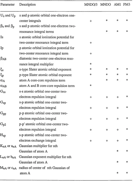
Table 1.1 shows the parameters that used in the four main methods and their nature. Parameters optimized for a given method are indicated by*. A+ indicates that the value of parameter was obtained from experiment (not optimized). The blanks mean that the

Table 1.1 Parameters used in the four main semiempirical methods and their natures

Parameter Description MND0/3 MNDO AM1 PM3

Us and Up s and p atomic orbital electron

one-center integrals ₊

*

*

*

~sand ~P s and p atomic orbital one-electron

two-resonance integral terms

*

*

*

Is s atomic orbital ionization potential for

two-center resonance integral term ₊ Ip p atomic orbital ionization potential for

two-center resonance integral term ₊

~AB diatomic two-center one-electron

reso-nance integral multiplier

*

~s s-type Slater atomic orbital exponent

*

*

*

*

~p p-type Slater atomic orbital exponent

*

*

*

*

a

*

*

*

aAB atom A and B core-core repulsion term

*

two-electron repulsion integral _{+ + +}

*

Gsp s-p atomic orbital one-center

two-electron repulsion integral ₊ + +

*

Gpp p-p atomic orbital one-center

two-electron repulsion integral _{+ +}

+

*

Gp2 p-p' atomic orbital one-center

two-electron repulsion integral _{+ + +}

*

Hsp s-p atomic orbital one-center

two-electron exchange integral _{+ +}

+

*

KnA or anA Gaussian multiplier for nth

Gaussian of atom A

*

*

LnA orbnA Gaussian exponent multiplier for nth

Gaussian of atom A

*

*

MnAOrCnA radius of center of nth Gaussian of

2.1 Introduction

Protonated diacetylene, C4H3+, has been found as a carbocation in acetylenic flame as a result of the reaction:

HCCH+HCCH HCCCCH2+ + H + other products (1)

The molecule C4H2 was also identified as one of the polyacetylenes which are constituents of interstellar clouds and primitive planetary atmospheres [79]. This molecule is likely to be protonated by H3+ and HCQ+, which are abundant in these ionizing

environments and can transfer protons to molecules with higher proton affinities (PAs).

HCCCCH +H3+

HCCCCH + HCQ+

HCCCCH2+ + H2

HCCCCH2+ + CO

The protonated diacetylene may then recombine with electrons or undergo ion-molecule reactions, including proton transfer to other ion-molecules having higher proton affinities. Thus the proton affinity is an important property for deciding subsequent chemical processes of diacetylene in the gas phase.

(2)

(3)

In the present study we used the Gaussian 82 [11] program to calculate a theoretical value of the proton affinity of diacetylene at the MP4SDQ level with a 6-3110** basis set. The calculated results were supported by selected ion flow tube (SIFf) measurements of proton transfer equilibria between diacetylene and C2Hsi, BrCN and CH3ND2 [101]. We also compare our results with the other calculations on diacetylene at different levels of

theory by Deakyne et al. [29] and Botschwina et al. [15]. Deakyne et al. [29] also performed experimental ion cycloton resonance (ICR) studies to confmn their theoretical results.

2.2 Theory

B

+

while gas phase basicity is defined as:

-~0(298)

=

+

In our study we compute the P A , using the formulae:

PA

=

~H(298)calcd

=

+

Definitions:

(4)

(5)

(6)

(7)

(8)

~ueo is the computed difference in the electronic energies of reactants and products at 0 K, including the correlation energy correction to the Hartree-Fock energy.

~(~Ue)298 is the change in the electronic energy difference between 298 K and 0 K. This term should be negligible for our study.

~uvo is the difference between the zero-point vibrational energies of reactants and product at 0 K.

~(~Uv)298 is the change in the vibrational energy difference between 298 and 0 K.

~Ur298 is the difference in rotational energies of reactants and product. Classically, this is equal to (-l/2)RT for each degree of rotational freedom lost during to the complex formation [84]. This value is equal to 0.0 in this study.

~Ut298 is the translational energy change due to the change in the number of degrees of freedom. In our study, three degree of freedom are lost by the hydrogen atom, so that this term is equal to (-3/2)RT.

~(PV), which is the PV work term at constant pressure, is the difference between

In order to calculate P A of C4H2, we need to identify the most stable structural isomer of C4H3+. The three lowest energies structures for C4H2 : vinylacetylene, methylene cyclopropane and cyclobutadiene were taken as starting species [68] . The structures (2) and (5) are generated by removal of hydrogen out of vinyl acetylene and ionizing the products. Methylenecyclopropene, after removal of methylene hydrogen and ionization, will give structure (3). The four-membered carbon 1ing isomer for C4H3+ is the bent structure (4). The planar four-membered ring structure (6) is a transition state and so gives one imaginruy frequency in our calculations.

1.055 1.185 1.387

H---c===c---c===c---H 4 - 3 2 - 1

(1)

H

11.065

c

154.1:! 1.247

138.0

1\

p

c~.010

H 1.269 H

(3)

1.062 1.186

(5)

H

1.064 1.275 1.323 1.203

~H

H-c=c-c===c~; 120.1 4 3 2 1'<.H 1.080

(2)

~.449

H ... c 75 ·7 c-H

~/

\r

: 1.073

H

(4)

c

~'-y-.124

1.011 / ₈

1.8

H-C~~:-

5

H

1.076

y

H (6)

were calculated at RHF level using the Gaussian 82 program with 6-31G* and 6-311G** basis sets. The correlation energies were calculated with fourth order M~ller-Plesset

perturbation theory, MP4SDQ, which includes contributions from single, double and quadruple excitations. The Harmonic vibration frequencies were calculated at the HF/6-31G* level and zero-point vibrational energies were determined. Following Pitzer [103], the contribution of the harmonically approximated, low-frequency vibrational modes at 298 K was evaluated as

(9)

where

u

=

(10) R = gas constant

Here v is the frequency (in cm-1) of the normal mode, and i and j range over product and

reactant normal modes respectively. The zero-point vibrational energies .1(AUv) value are multiplied by a scale factor of 0.89 as suggested by DeFrees and Pople [109].

2.4 Results

parameters HF HF CEPA-1 HF 6-311G**a 6-31G**b n-cGTQsc n-cGTQsd

C4H2

r12 1.185 1.188 1.211

r23 1.387 1.389 1.380

rcH 1.055 1.057 1.060

C4H3+

r12 1.203 1.207 1.230 1.200

r23 1.323 1.325 1.321 1.321

r34 1.275 1.278 1.292 1.271

r1H 1.081 1.081 1.088 1.079

f4H 1.064 1.066 1.070 1.062

ARcH 120.1 120.0 119.1 120.1

a This work, using GAUSSIAN 82.

b Deakyne et al. [29], using GAUSSIAN 82.

c Botschwina et al. [15], using Meyer's Coupled Electron Pair Approximation method, 96 cGTOs for C4H2 and 102 cGTOs for C4H3+

Structure HF MP2 MP4SDQ ZPVE Hartree

6-310* Basis set

(1) C4H2 -152.49793 -153.00760 -153.00602 0.042006 (2) C4H3+ -152.79842 -153.28728 -153.29621 0.050784 (3) -152.77082 -153.25617 -153.26555 0.050265 (4) -152.76789 -153.24629 -153.25724 0.053400 (5) -152.75413 -153.23287 -153.24548 0.050209 (6) -152.73325 -153.19350 -153.26555 0.050265 6-3110** Basis set

(1) C4H2 -152.53525 -153.07111

(2) C4H3+ -153.83117 -153.35909

Table 2.3 Calculated electronic energies with zero-point vibrational energies correction (kJ mol-l).

Structure

6-310* Basis set (1).C4H2

(2) C4H3+ (3)

(4) (5) (6)

6-3110** Basis set

0.0 -738.8 -659.7 -629.7 -607.2 -506.0

0.0 -733.oa

MP4SDQ

6-311G**b -756.08092 -733.03428 -3.54666 with 0.89d

correction -756.08092 -735.56941 -3.82310e MP3

6-31G**f -777.3872 -759.8144 -5.0208

CEPA-1g -756.5 -736.7 -4.5

a temperature contribution= il(ilUv)298 + ~Ut298 + ~Ur298 +

MV

c Reference101

(PAexp)

736.58093

739.39251 (741

±

±

d 0.89 factor for calculated vibrational results suggested by Defrees and Pople [110]. e In this value, only ~(~Uv)298 was multiplied by 0.89.

f Work done by Deakyne et al. [29], experiment done on Ion Cycloton Resonance method. g Work done by Botschwina et al.[15], 130 and 124 contracted GTOs were used for C4H3+

Hartree-Pock Hartree-Fock CEP A -1 potential

6-310* basisa 3-210 basisb with vibrational

Hamiltonianc

(bz) 215 (bt) 219

(bt) 233 (bz) 224

(bz) 473 (bz) 535

(bt) 573 (bt) 587

(bt) 786 (bl) 880

(at) 960 (854) (at) 963 (at) 889

(bz) 997 (bz) 1059

(bz) 1032 (bz) 1107

(bt) 1075 (bt) 1122

(at) 1475 (1313) (at) 1501 (at) 1331

(at) 1975 (1758) (at) 1971 (at) 1789

(at) 2330 (2074) (at) 2261 (at) 2030

(at) 3294 (2932) (at) 3249 (at) 3045

(bz) 3392 (bz) 3336

(at) 3581 (3187) (at) 3547 (at) 3286

a This work, in bracket are the calculated vibrational frequencies multiplied by 0.89 factor. b Reference 29, the values were also suggested to multiplied with 0.89 factor to be compare

with experiment.

In this study we used the valence-double-split polarized basis 6-31G* and the valence-triple-split poladzed 6-311G** basis in the molecular orbital theory calculations. These basis sets should be sui