http://go.warwick.ac.uk/lib-publications
Original citation:
Abdallah, J., et al. (2011). A study of the b-quark fragmentation function with the DELPHI
detector at LEP I and an averaged distribution obtained at the Z Pole. The European
Physical Journal C, 71(2), article no. 1557.
Permanent WRAP url:
http://wrap.warwick.ac.uk/40102
Copyright and reuse:
The Warwick Research Archive Portal (WRAP) makes the work of researchers of the
University of Warwick available open access under the following conditions.
This article is made available under the Creative Commons
Attribution-NonCommercial-NoDerivs 3.0 Unported (CC BY-NC-ND 3.0) license and may be reused according to the
conditions of the license. For more details see:
http://creativecommons.org/licenses/by-nc-nd/3.0/
A note on versions:
The version presented in WRAP is the published version, or, version of record, and may
be cited as it appears here.
DOI 10.1140/epjc/s10052-011-1557-x
Regular Article - Experimental Physics
A study of the b-quark fragmentation function
with the DELPHI detector at LEP I and an averaged distribution
obtained at the Z Pole
The DELPHI Collaboration
J. Abdallah26, P. Abreu23, W. Adam55, P. Adzic12, T. Albrecht18, R. Alemany-Fernandez10, T. Allmendinger18, P.P. Allport24, U. Amaldi30, N. Amapane48, S. Amato52, E. Anashkin37, A. Andreazza29, S. Andringa23, N. Anjos23, P. Antilogus26, W-D. Apel18, Y. Arnoud15, S. Ask10, B. Asman47, J.E. Augustin26, A. Augustinus10, P. Baillon10,
A. Ballestrero49, P. Bambade21, R. Barbier28, D. Bardin17, G.J. Barkerd, A. Baroncelli40, M. Battaglia10, M. Baubillier26, K-H. Becks57, M. Begalli8, A. Behrmann57, E. Ben-Haim26, N. Benekos33, A. Benvenuti6, C. Berat15, M. Berggren26, D. Bertrand3, M. Besancon41, N. Besson41, D. Bloch11, M. Blom32, M. Bluj56, M. Bonesini30, M. Boonekamp41, P.S.L. Booth24,b, G. Borisov22, O. Botner53, B. Bouquet21, T.J.V. Bowcock24, I. Boyko17, M. Bracko44, R. Brenner53, E. Brodet36, P. Bruckman19, J.M. Brunet9, B. Buschbeck55, P. Buschmann57, M. Calvi30, T. Camporesi10, V. Canale39, F. Carena10, N. Castro23, F. Cavallo6, M. Chapkin43, Ph. Charpentier10, P. Checchia37, R. Chierici10, P. Chliapnikov43, J. Chudoba10, S.U. Chung10, K. Cieslik19, P. Collins10, R. Contri14, G. Cosme21, F. Cossutti50, M.J. Costa54, D. Crennell38, J. Cuevas35, J. D’Hondt3, T. da Silva52, W. Da Silva26, G. Della Ricca50, A. De Angelis51, W. De Boer18, C. De Clercq3, B. De Lotto51, N. De Maria48, A. De Min37, L. de Paula52, L. Di Ciaccio39, A. Di Simone40, K. Doroba56, J. Drees57,10, G. Eigen5, T. Ekelof53, M. Ellert53, M. Elsing10, M.C. Espirito Santo23, G. Fanourakis12, D. Fassouliotis12,4, M. Feindt18, J. Fernandez42, A. Ferrer54, F. Ferro14, U. Flagmeyer57, H. Foeth10, E. Fokitis33, F. Fulda-Quenzer21, J. Fuster54, M. Gandelman52, C. Garcia54, Ph. Gavillet10, E. Gazis33, R. Gokieli10,56, B. Golob44,46, G. Gomez-Ceballos42, P. Goncalves23, E. Graziani40,
G. Grosdidier21, K. Grzelak56, J. Guy38, C. Haag18, A. Hallgren53, K. Hamacher57, K. Hamilton36, S. Haug34, F. Hauler18, V. Hedberg27, M. Hennecke18, J. Hoffman56, S-O. Holmgren47, P.J. Holt10, M.A. Houlden24,
J.N. Jackson24, G. Jarlskog27, P. Jarry41, D. Jeans36, E.K. Johansson47, P. Jonsson28, C. Joram10, L. Jungermann18,
F. Kapusta26, S. Katsanevas28, E. Katsoufis33, G. Kernel44, B.P. Kersevan44,46, U. Kerzel18, B.T. King24, N.J. Kjaer10, P. Kluit32, P. Kokkinias12, C. Kourkoumelis4, O. Kouznetsov17, Z. Krumstein17, M. Kucharczyk19, J. Lamsa1, G. Leder55, F. Ledroit15, L. Leinonen47, R. Leitner31, J. Lemonne3, V. Lepeltier21,b, T. Lesiak19, W. Liebig57, D. Liko55, A. Lipniacka47, J.H. Lopes52, J.M. Lopez35, D. Loukas12, P. Lutz41, L. Lyons36, J. MacNaughton55, A. Malek57, S. Maltezos33, F. Mandl55, J. Marco42, R. Marco42, B. Marechal52, M. Margoni37, J-C. Marin10, C. Mariotti10, A. Markou12, C. Martinez-Rivero42, J. Masik13, N. Mastroyiannopoulos12, F. Matorras42, C. Matteuzzi30, F. Mazzucato37, M. Mazzucato37, R. Mc Nulty24, C. Meroni29, E. Migliore48, W. Mitaroff55, U. Mjoernmark27, T. Moa47, M. Moch18, K. Moenig10,c, R. Monge14, J. Montenegro32, D. Moraes52, S. Moreno23, P. Morettini14, U. Mueller57, K. Muenich57, M. Mulders32, L. Mundim8, W. Murray38, B. Muryn20, G. Myatt36, T. Myklebust34, M. Nassiakou12, F. Navarria6, K. Nawrocki56, S. Nemecek13, R. Nicolaidou41, M. Nikolenko17,11, A. Oblakowska-Mucha20, V. Obraztsov43, A. Olshevski17, A. Onofre23, R. Orava16, K. Osterberg16, A. Ouraou41, A. Oyanguren54, M. Paganoni30, S. Paiano6, J.P. Palacios24, H. Palka19, Th.D. Papadopoulou33, L. Pape10, C. Parkes25, F. Parodi14, U. Parzefall10, A. Passeri40, O. Passon57, L. Peralta23, V. Perepelitsa54, A. Perrotta6,
A. Petrolini14, J. Piedra42, L. Pieri40, F. Pierre41,b, M. Pimenta23, E. Piotto10, T. Podobnik44,46, V. Poireau10, M.E. Pol7, G. Polok19, V. Pozdniakov17, N. Pukhaeva17, A. Pullia30, D. Radojicic36, P. Rebecchi10, J. Rehn18, D. Reid32, R. Reinhardt57, P. Renton36, F. Richard21, J. Ridky13, M. Rivero42, D. Rodriguez42, A. Romero48,
W. Venus38, P. Verdier28, V. Verzi39, D. Vilanova41, L. Vitale50, V. Vrba13, H. Wahlen57, A.J. Washbrook24, C. Weiser18, D. Wicke10, J. Wickens3, G. Wilkinson36, M. Winter11, M. Witek19, O. Yushchenko43, A. Zalewska19, P. Zalewski56, D. Zavrtanik45, V. Zhuravlov17, N.I. Zimin17, A. Zintchenko17, M. Zupan12
1
Department of Physics and Astronomy, Iowa State University, Ames, IA 50011-3160, USA 2
Physics Department, Universiteit Antwerpen, Universiteitsplein 1, 2610 Antwerpen, Belgium 3
IIHE, ULB-VUB, Pleinlaan 2, 1050 Brussels, Belgium 4
Physics Laboratory, University of Athens, Solonos Str. 104, 10680 Athens, Greece 5
Department of Physics, University of Bergen, Allégaten 55, 5007 Bergen, Norway
6Dipartimento di Fisica, Università di Bologna and INFN, Viale C. Berti Pichat 6/2, 40127 Bologna, Italy 7Centro Brasileiro de Pesquisas Físicas, rua Xavier Sigaud 150, 22290 Rio de Janeiro, Brazil
8Inst. de Física, Univ. Estadual do Rio de Janeiro, rua São Francisco Xavier 524, Rio de Janeiro, Brazil 9
Collège de France, Lab. de Physique Corpusculaire, IN2P3-CNRS, 75231 Paris Cedex 05, France 10
CERN, 1211 Geneva 23, Switzerland 11
Institut Pluridisciplinaire Hubert Curien, Université de Strasbourg, IN2P3-CNRS, BP28, 67037 Strasbourg Cedex 2, France 12
Institute of Nuclear Physics, N.C.S.R. Demokritos, P.O. Box 60228, 15310 Athens, Greece 13
FZU, Inst. of Phys. of the C.A.S. High Energy Physics Division, Na Slovance 2, 182 21, Praha 8, Czech Republic 14
Dipartimento di Fisica, Università di Genova and INFN, Via Dodecaneso 33, 16146 Genova, Italy 15
Institut des Sciences Nucléaires, IN2P3-CNRS, Université de Grenoble 1, 38026 Grenoble Cedex, France 16
Helsinki Institute of Physics and Department of Physical Sciences, P.O. Box 64, 00014 University of Helsinki, Finland 17
Joint Institute for Nuclear Research, Dubna, Head Post Office, P.O. Box 79, 101 000 Moscow, Russian Federation 18
Institut für Experimentelle Kernphysik, Universität Karlsruhe, Postfach 6980, 76128 Karlsruhe, Germany 19
Institute of Nuclear Physics PAN, Ul. Radzikowskiego 152, 31142 Krakow, Poland 20
Faculty of Physics and Nuclear Techniques, University of Mining and Metallurgy, 30055 Krakow, Poland 21
LAL, Univ Paris-Sud, CNRS/IN2P3, Orsay, France 22
School of Physics and Chemistry, University of Lancaster, Lancaster LA1 4YB, UK 23
LIP, IST, FCUL, Av. Elias Garcia, 14-1°, 1000 Lisboa Codex, Portugal
24Department of Physics, University of Liverpool, P.O. Box 147, Liverpool L69 3BX, UK
25Dept. of Physics and Astronomy, Kelvin Building, University of Glasgow, Glasgow G12 8QQ, UK
26LPNHE, Univ. Pierre et Marie Curie, Univ. Paris Diderot, CNRS/IN2P3, 4 pl. Jussieu, 75252 Paris Cedex 05, France 27
Department of Physics, University of Lund, Sölvegatan 14, 223 63 Lund, Sweden 28
Université Claude Bernard de Lyon, IPNL, IN2P3-CNRS, 69622 Villeurbanne Cedex, France 29
Dipartimento di Fisica, Università di Milano and INFN-MILANO, Via Celoria 16, 20133 Milan, Italy 30
Dipartimento di Fisica, Univ. di Milano-Bicocca and INFN-MILANO, Piazza della Scienza 3, 20126 Milan, Italy 31
IPNP of MFF, Charles Univ., Areal MFF, V Holesovickach 2, 180 00, Praha 8, Czech Republic 32
NIKHEF, Postbus 41882, 1009 DB Amsterdam, The Netherlands 33
National Technical University, Physics Department, Zografou Campus, 15773 Athens, Greece 34
Physics Department, University of Oslo, Blindern, 0316 Oslo, Norway 35
Dpto. Fisica, Univ. Oviedo, Avda. Calvo Sotelo s/n, 33007 Oviedo, Spain 36
Department of Physics, University of Oxford, Keble Road, Oxford OX1 3RH, UK 37
Dipartimento di Fisica, Università di Padova and INFN, Via Marzolo 8, 35131 Padua, Italy 38
Rutherford Appleton Laboratory, Chilton, Didcot OX11 OQX, UK 39
Dipartimento di Fisica, Università di Roma II and INFN, Tor Vergata, 00173 Rome, Italy 40
Dipartimento di Fisica, Università di Roma III and INFN, Via della Vasca Navale 84, 00146 Rome, Italy 41
DAPNIA/Service de Physique des Particules, CEA-Saclay, 91191 Gif-sur-Yvette Cedex, France 42Instituto de Fisica de Cantabria (CSIC-UC), Avda. los Castros s/n, 39006 Santander, Spain
43Inst. for High Energy Physics, Serpukov P.O. Box 35, Protvino, Moscow Region, Russian Federation 44J. Stefan Institute, Jamova 39, 1000 Ljubljana, Slovenia
45
Laboratory for Astroparticle Physics, University of Nova Gorica, Kostanjeviska 16a, 5000 Nova Gorica, Slovenia 46
Department of Physics, University of Ljubljana, 1000 Ljubljana, Slovenia 47
Fysikum, Stockholm University, Box 6730, 113 85 Stockholm, Sweden 48
Dipartimento di Fisica Sperimentale, Università di Torino and INFN, Via P. Giuria 1, 10125 Turin, Italy 49
INFN, Sezione di Torino and Dipartimento di Fisica Teorica, Università di Torino, Via Giuria 1, 10125 Turin, Italy 50
Dipartimento di Fisica, Università di Trieste and INFN, Via A. Valerio 2, 34127 Trieste, Italy 51
Istituto di Fisica, Università di Udine and INFN, 33100 Udine, Italy 52
Univ. Federal do Rio de Janeiro, C.P. 68528 Cidade Univ., Ilha do Fundão, 21945-970 Rio de Janeiro, Brazil 53
Department of Radiation Sciences, University of Uppsala, P.O. Box 535, 751 21 Uppsala, Sweden 54
IFIC, Valencia-CSIC, and D.F.A.M.N., U. de Valencia, Avda. Dr. Moliner 50, 46100 Burjassot, Valencia, Spain 55
Institut für Hochenergiephysik, Österr. Akad. d. Wissensch., Nikolsdorfergasse 18, 1050 Vienna, Austria 56
Inst. Nuclear Studies and University of Warsaw, Ul. Hoza 69, 00681 Warsaw, Poland 57
Fachbereich Physik, University of Wuppertal, Postfach 100 127, 42097 Wuppertal, Germany
Abstract The nature of b-quark jet hadronisation has been investigated using data taken at the Z peak by the DELPHI detector at LEP. Two complementary methods are used to re-construct the energy of weakly decaying b-hadrons,EBweak. The average value ofxBweak=EweakB /Ebeamis measured to be 0.699±0.011. The resultingxBweak distribution is then analysed in the framework of two choices for the perturba-tive contribution (parton shower and Next to Leading Log QCD calculation) in order to extract measurements of the non-perturbative contribution to be used in studies of b-hadron production in other experimental environments than LEP. In the parton shower framework, data favour the Lund model ansatz and corresponding values of its parameters have been determined within PYTHIA 6.156 from DELPHI data:
a=1.84+−00..2321 and b=0.642+−00..073063GeV−2,
with a correlation factorρ=92.2%.
Combining the data on the b-quark fragmentation dis-tributions with those obtained at the Z peak by ALEPH, OPAL and SLD, the average value of xBweak is found to be 0.7092±0.0025 and the non-perturbative fragmentation component is extracted. Using the combined distribution, a better determination of the Lund parameters is also ob-tained:
a=1.48+−00..1110 and b=0.509+−00..024023GeV−2,
with a correlation factorρ=92.6%.
1 Introduction and overview
The fragmentation of a bb quark pair from Z decay, into jets of particles including the parent b-quarks bound inside b-hadrons, is a process that can be viewed in two stages. The first stage involves the b-quarks radiating hard gluons at scales ofQ2Λ2QCDfor which the strong coupling is small αs1. These gluons can themselves split into further glu-ons or quark pairs in a kind of ‘parton shower’. By virtue of the small coupling, this stage can be described by perturba-tive QCD implemented either as exact QCD matrix elements or leading-log parton shower cascade models in event gen-erators. As the partons separate, the energy scale drops to ∼Λ2QCDand the strong coupling becomes large, correspond-ing to a regime where perturbation theory no longer applies. Through the self interaction of radiated gluons, the colour
ae-mail:[email protected] bDeceased.
cNow at DESY-Zeuthen, Platanenallee 6, 15735 Zeuthen, Germany. dNow at Department of Physics, University of Warwick, Coventry CV4 7AL, UK.
field energy density between partons builds up to the point where there is sufficient energy to create new quark pairs from the vacuum. This process continues with the result that colourless clusters of quarks and gluons with low internal momentum become bound up together to form hadrons. This ‘hadronisation’ process represents the second stage of the b-quark fragmentation which cannot be calculated in perturba-tion theory and must be modelled in some way. In simulaperturba-tion programs this is made via a ‘fragmentation function’ which, in the case of b-hadron production, parameterises how en-ergy/momentum is shared between the parent b-quark and its final state b-hadron. Important steps for the understand-ing of the hadronisation mechanism are given in references [1–4].
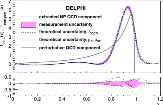
The purpose of this study is to measure the non-perturb-ative contribution to b-quark fragmentation in a way that is independent of any non-perturbative hadronisation model. Up to the choice of either QCD matrix element or leading-log parton shower to represent the perturbative phase, results are obtained that are applicable to any b-hadron production environment in addition to the Z→bb data on which the measurements were made.
Results from two analyses are reported which measure the b-quark fragmentation function from the data taken in 1994 by the DELPHI detector at LEP. Several definitions of the functions and variables used in the measurement of the b-quark fragmentation distribution are given in Sect.2. Section3contains a short description of the DELPHI detec-tor with emphasis on components which are relevant for the present measurement. Section4describes how two different approaches (Regularised Unfolding and Weighted Fitting) have been used to extract from the data the underlying en-ergy distribution of weakly decaying b-hadrons. These mea-surements are then combined in Sect. 4.3 and interpreted (in Sect. 5) as the combined result of a perturbative and a non-perturbative part. Corresponding fragmentation func-tions are determined by (a) finding the best fit to the data with a full simulation of the hadronisation process, where the perturbative contribution is made by a parton shower model, and (b) by describing the perturbative part with a NLL QCD calculation and using the inverse Mellin transfor-mation to solve for the non-perturbative part. Present mea-surements are combined in Sect.6with previous experimen-tal results to obtain a world averaged b-quark fragmentation distribution.
2 Fragmentation functions
DbB(v)(parameterised in terms of some kinematical variable v), which can be interpreted as the probability density func-tion that a hadron B, containing the original quark b, is pro-duced with a given value ofv. In order to reproduce the data accurately, the fragmentation function must have an appro-priate form with parameters that are tuned to the data.
Although the definition ofvvaries from model to model, generally speaking it is a quantity that reflects the fraction of the available energy that the b-hadron receives from the hadronisation process. For models relevant to b-quark frag-mentation from Z decay, the choice of fragfrag-mentation vari-ablevusually falls into one of two broad categories: • zis a fraction normalised to kinematical properties of the
parent b-quark just before the hadronisation process be-gins;
• x is a fraction normalised to the electron/positron beam energy i.e.√s/2.
From a phenomenological point of view, z is the relevant choice of variable for a parameterisation implemented in an event generator algorithm. However, becausezdepends ex-plicitly on the properties of the parent b-quark, it is not a quantity that can be directly measured by experiments. For this reason all existing measurements ofDbB(v)are based on the reconstruction ofx.
Throughout this paper, the Lund fragmentation model [5] definition of z is employed. In the Lund model, hadroni-sation is described by breaks in a string linking two par-tons which mimics the colour field energy density between them crossing the threshold for the creation of a new quark pair. The fragmentation variable, for the case of an initial bb quark system in the absence of gluon radiation, is defined as
z=(E+p||)B (E+p)b
. (1)
Here,p|| represents the hadron momentum in the direction of the b-quark and(E+p)b is the sum of the energy and momentum of the b-quark just before fragmentation begins. When discussingx, it is necessary to be clear about ex-actly which hadron is being considered. The primary b-hadron is the state created directly after the b-hadronisation phase, whereas the weakly decaying b-hadron is the state that finally decays somewhere in the detector volume in a flavour-changing process. Primary b-hadrons are either mesons (about 90%) or baryons (about 10%) [6]. In the case of mesons, measurements suggest that about 25% of primary b-hadrons are orbitally excited B∗∗ mesons [7,8], about 52% are B∗ mesons and only about 18% are weakly decaying B+,B0dor B0s mesons [9–11]. B∗∗and B∗mesons decay via kaon, pion or photon emission into weakly de-caying ground state mesons, which then carry less energy than their parents. For both analyses presented here, the b-hadron under consideration is always the weakly decaying
state. Two choices for thex fragmentation variable in com-mon use arexBweakandxpweak:
xBweak=E
weak B
Eb
(2)
is the fraction of the energy taken by the b-hadron with re-spect to the energy of the b-quark directly after its produc-tion i.e. before any gluons have been radiated. This defini-tion is particularly suited toe+e− annihilation as both the numerator and denominator are directly observable. This follows since, in the absence of initial state radiation, the quark energy is equal to the electron beam energy:
xBweak=2E
weak B √
s =
EBweak
Ebeam
. (3)
The variablexpweakis defined as the ratio of the three mo-menta (p) which, assumingmB=mb, can be expressed as,
xpweak= p
weak B
pweakB,max=
xBweak2−xmin2
1−xmin2
(4)
where xmin= 2√msB is the minimum value of xBweak and
pweakB,max is the maximum momentum taken by the b-hadron assuming that its energy is equal to the beam energy.
3 The DELPHI detector and b-tagging
A complete overview of the DELPHI detector and its per-formance have been described elsewhere [12,13]. What fol-lows is a short description of the elements most relevant to this analysis.
In the barrel region, charged particle tracking was per-formed by the Vertex Detector (VD), the Inner Detector, the Time Projection Chamber (TPC) and the Outer Detector. In the end-cap regions, two sets of drift chambers (FCA and FCB) were situated at about 160 cm and 275 cm from the interaction point (IP) respectively. They covered polar an-gles,θ, in the range[11◦,36◦]and[144◦, 169◦].1A highly uniform magnetic field of 1.23 T parallel to thee+e−beam direction, was provided by the superconducting solenoid throughout the tracking volume. The momentum of charged particles was measured with a precision ofσp/p≤1.5% in the θ region [40◦, 140◦] and forp <10 GeV/c. The VD consisted of three layers of silicon micro-strip devices with
an intrinsic resolution of about 8 µm in theR–φplane trans-verse to the beam line. In addition, the inner- and outer-most layers were instrumented with double-sided devices providing coordinates of similar precision in theRZ plane along the direction of the beams. For charged particles with hits in all three Rφ VD layers the impact parameter res-olution wasσRφ2 =([61/(psin3/2θ )]2+202)µm2and for tracks with hits in bothRZlayers and withθ≈90◦,σRZ2 = ([67/(psin5/2θ )]2+332)µm2(pis in GeV/c).
Calorimeters detected photons and neutral hadrons by the total absorption of their energy. The High-density Projec-tion Chamber (HPC) provided electromagnetic calorimetry coverage in the region 46◦< θ <134◦giving a relative pre-cision on the measured energyE of σE/E=0.32/
√ E⊕ 0.043 (E in GeV). In addition, each HPC module worked essentially as a small TPC charting the spatial development of showers and so providing an improved angular resolu-tion, which is better than that from the detector granular-ity alone. For high energy photons the angular precisions were±1.7 mrad in the azimuthal angleφand±1.0 mrad in θ. The Forward Electromagnetic Calorimeter consisted of two arrays of 4532 Cherenkov lead glass blocks with 20 ra-diation lengths. The front faces of the blocks were placed at ±284 cm from the IP, covering the polar angle in the ranges [8◦, 35◦] and[145◦, 172◦]. The relative precision on the measured energy could be parameterised asσE/E= 0.03⊕0.12/√E⊕0.11/E(Ein GeV). For neutral show-ers of energy larger than 2 GeV, the average precision on the reconstructed hit position in X and Y was about 0.5 cm. The Hadron Calorimeter was installed in the return yoke of the DELPHI solenoid and provided a relative precision on the measured energy ofσE/E=1.12/
√
E⊕0.21 (Ein GeV). Powerful particle identification was made possible by the combination ofdE/dx information from the TPC (and to a lesser extent from the VD) with information from the Ring Imaging CHerenkov counters (RICH) in both the forward and barrel regions. The RICH devices utilised both liquid and gas radiators in order to optimise coverage across a wide momentum range: liquid was used for the momentum range from 0.7 GeV/cto 8 GeV/cand the gas radiator for the range 2.5 GeV/cto 25 GeV/c.
The impact parameters provided the main variable for b-tagging. For all the charged particle tracks in the jet, the im-pact parameters and resolutions were combined into a sin-gle variable, the lifetime probability, which measured the consistency with the hypothesis that all tracks come directly from the primary vertex. For events without long-lived par-ticles, this variable should be uniformly distributed between zero and unity. In contrast, for b-jets it has predominantly small values. This information is used in the weighted fitting algorithm whereas additional characteristics of bb-events are included in the other approach. Other features of the event are also sensitive to the presence of b-quarks, and
some of them are used together with the impact parameters information to construct a ‘combined’ tag. For example, b-hadrons have a 10% probability of decaying to electrons or muons, and these often have a transverse momentum with respect to the b-jet axis of around 1 GeV/cor larger. The combined tag also makes use of other variables that have significantly different distributions for b-quark and for other events, e.g. the charged particle rapidities with respect to the jet axis. Further details on the b-tagging algorithm can be found in reference [14].
In the analyses described in this paper, the primary and the secondary vertices are reconstructed in 3 dimensions.
4 Measuringf (xBweak)
This paper describes two independent methods of recon-structingxBweakfrom the data: one which unfolds the under-lying physics distribution from the measured quantity and one which fits for the physics distribution by a weighting technique. The former is described in Sect.4.1and the latter in Sect.4.2. The two methods differ also in the way parti-cles are classified as originating from a b-hadron decay or from fragmentation. The first method is using extensively Neural Networks whereas the second is based on different techniques. Both methods are independent of any initial as-sumption regarding the actual shape of the underlying frag-mentation function in simulation. Throughout this section all charged particles are assumed to be pions, and for pho-tons and neutral hadrons we use the candidates measured in calorimeters as described in Sect.3.
4.1 The regularised unfolding analysis
The experimental challenge of this method is to deter-mine from the measured distribution in data2 g(xweakB,rec), the underlying fragmentation functionf (xBweak). In general g(xBweak,rec)will differ fromf (xBweak)due to:
(a) finite detector resolution; (b) limited measurement acceptance;
(c) variable transformation, i.e. any biases or distortions that may be present in the measured quantity.
Mathematically, the distributions are related by:
gxBweak,rec=
RxBweak,rec;xBweakfxBweakdxBweak+bxBweak,rec,
(5)
Table 1 Details of the event
generator used together with some of the more relevant parameter values that have been tuned to the DELPHI data
Event Generator JETSET 7.3 [15,16]
Perturbative ansatz Parton shower (ΛQCD=0.346 GeV,Q0=2.25 GeV) [17] Non-perturbative ansatz String fragmentation
Fragmentation function Peterson [18] (b=0.002326) Bose–Einstein correlations Enabled
whereR(xweakB,rec;xBweak)is the response function which de-scribes the mapping ofxBweak,reconto truexBweakand thus con-tains all the effects of resolution, acceptance and variable transformation mentioned above. The term b(xBweak,rec)is the background contribution and is taken from simulation.
4.1.1 Hadronic event selection
Hadronic Z decays were selected by the following require-ments:
(a) at least 5 reconstructed charged particles;
(b) the summed energy in charged particles with momen-tum greater than 0.2 GeV/chad to be larger than 12% of the centre-of-mass energy, with at least 3% of it in each of the forward and backward hemispheres defined with respect to the beam axis.
These requirements resulted in the selection of about 1.36 million events from data. The simulated sample of Z→ qq events, details of which are listed in Table1, contained approximately three times the number of data events. The generated events were passed through a full detector simu-lation [13] and the same multihadronic selection criteria as the data.
4.1.2 Event hemisphere selection
In each event, particles are distributed in two hemispheres depending on their direction relative to the thrust axis. Event hemispheres used for the analysis were accepted if the fol-lowing criteria were fulfilled:
(a) |cosθthrust|<0.7, whereθthrustis the polar angle of the event thrust axis relative to the beam direction;
(b) the hemisphere was tagged as a Z→bb candidate event by the standard DELPHI b-tagging package [14]; (c) the secondary vertex fit converged successfully; (d) 0.5< Ehem/Ebeam<1.1 where Ehem is equal to the
sum of the energy of particles contained in the hemi-sphere.
After this selection, 227940 hemispheres remained in the data with a purity (as calculated from the simulation) in bb events of 96%.
4.1.3 The reconstruction ofEBweak
The following corrections were applied to the simulation to account for known discrepancies with the data which could affect modelling of the B-energy scale:
(a) The reconstructed energy distributions per charged or neutral particle were separately shifted and smeared3in the simulation to bring them into better agreement with the data (based on aχ2-histogram comparison). (b) The multiplicities of:
– fragmentation charged particles (identified by a selec-tion cut on the TrackNet4<0.5),
– b-hadron weak decay products (identified by a selec-tion cut on the TrackNet>0.5),
– neutral particles,
were fixed separately in the simulation by a weighting function, to agree with the data.
(c) After applying the above two corrections, a very small residual difference remained between data and simula-tion in the total energy of charged particles (“charged energy”) and neutral particles (“neutral energy”) which was accounted for by a further weighting function.
The energyEBweak of a b-hadron undergoing weak de-cay within the hemisphere of a Z hadronic-dede-cay event, was reconstructed using the Neural Network (NN) package, Neurobayes [19]. The full list of variables that the NN was trained on is presented in AppendixA. Since the degree of correlation of the inputs to the network target value natu-rally varies from case to case, a pre-processing stage to the network algorithm was used to suppress the influence of the inputs with low correlation automatically and so retain opti-mal performance. The network was trained to return a com-plete probability density function (p.d.f.) for the energy, on a hemisphere-by-hemisphere basis, andEweakB was defined to be the median of this distribution. Full details of this ap-proach can be found in reference [19].
3For charged particles the shift in the mean was 0.01 GeV and a Gaussian smearing of 3% (relative) applied. For neutral clusters the corresponding numbers were 0.04 GeV and 20%.
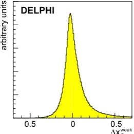
The precision of the resulting estimator, based on a statis-tically independent simulated event sample to that used for training and after all analysis selection cuts have been ap-plied, is shown in Fig.1. The full width at half maximum is 14.0%.
4.1.4 The unfolding method
The solution of (5) for f (xBweak) is a non-trivial problem since the solution can be highly oscillatory. A practical solu-tion to this is provided by the RUN(Regularised UNfolding) program [20] which applies regularisation techniques to im-pose the condition that the solution must be smooth. In prac-tice, the algorithm defines a functionW (xBweak)used to pro-vide a weight to the simulated distributiongsim(xweakB,rec)such that it reproduces the data distribution g(xBweak,rec)as well as possible, i.e. W (xBweak) is determined by a fit to the data. The result of the unfolding, up to a normalisation factor, is then given by
fxBweak=WxBweak·fsim
xBweak (6)
wherefsim(xBweak)is the fragmentation function used to gen-erate the simulated events. By summing over bins inxBweak, unfolded binned points are determined together with a com-plete covariance matrix.
It is important to note that internally to RUN, the weight factors are defined as a sum over orthogonal polynomials taken to be basis splinesP (xBweak),
WxBweak= m
j=1
aj·Pj
xBweak (7)
[image:8.595.105.236.548.679.2]whereaj are suitable expansion coefficients. Consequently, the difficult task of solving (5) reduces to deciding at which point to cutoff the sum in (7). This point,j=m, is referred to in what follows as the number of degrees of freedom of the unfolding procedure. Full details of the unfolding method can be found in reference [21].
Fig. 1 Distribution of the precision of the NN estimator forxBweak, defined asxBweak=(xBweak,rec−xBweak,gen)/xBweak,gen
4.1.5 Unfolding results
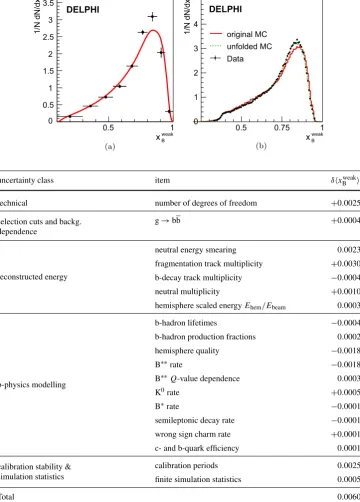
The result of the unfolding applied to the real data set is displayed in Fig.2a. The plot shows the unfolded, binned, data points together with an overlay of the ‘truth’ or gen-eratedf (xBweak)distribution that is the input to the detector simulation. The binning of the unfolded points was chosen to match the observed resolution inxBweakaccording to the measurement uncertainties described in Sect.4.1.3. For the case ofxBweakthe median (relative) error varied from about 5% at anxBweak value close to 1.0 and degraded to about 65% atxBweak=0.2. The number of degrees of freedom in the unfolding procedure was chosen to be as low as possible (i.e. five) in order to ensure a smooth result. The lower limit is constrained by the need to include all terms in the sum-mation (7) for which the size of the expansion coefficients aj are significant.
The results show that there is a basic disagreement in shape between the distribution unfolded from data and the corresponding truth distribution from the simulation before the application of weights. Figure2b shows the excellent agreement that exists between data and simulation after appropriately weighting the generator distribution to agree with the result of the unfolding.
In order to quantify the shape of the unfolded distribu-tion, the mean (x =01xf (x) dx) and variance (σ2(x)=
1
0(x− x)
2f (x) dx) have been calculated and the results
were: xBweak =0.7140±0.0007(stat.) and σ2(xBweak)= 0.0308±0.0003(stat.). The mean value quoted has been corrected to account for the effect of Initial State Radia-tion (ISR) which is necessary sincex is formed by scaling EweakB by the nominal beam energy of 45.6 GeV. This is only strictly correct in the case of no ISR and in about 10% of cases ISR reduces the energy available for the fragmenting b-quark system from the nominal value. The size of this ef-fect on the analysis was evaluated from the simulation and the resulting mean value forEBweakwas shifted by+50 MeV. The corresponding shift ofxBweakisδxBweak = +0.0011. The full bin-to-bin unfolding results including covariance matrices, are listed in AppendixB.
4.1.6 Systematic uncertainties
Systematic uncertainties on the unfolded distribution of xBweak have been evaluated from a wide variety of sources, the effects of which onxBweakare presented in Table2. In addition, statistical and systematic uncertainties for each of the nine unfolded bins of Fig.2a are given in AppendixB
together with the associated covariance matrices.
Fig. 2 (a) The result of
unfoldingxBweakfrom real data (points), and the generator-level fsim(xweakB )distribution, before applying weights (curve). (b) Distribution ofxBweakin the data,g(xBweak,rec), compared to both the default simulation gsim(xBweak,rec)and the simulation weighted for the results of the fragmentation function unfolding result shown in (a)
Table 2 Systematic uncertainty
on the mean value of the unfoldedxBweakdistribution. The total is the sum in quadrature of all contributions. The sign indicates the correlation between the change in an uncertainty source and the shift in the final result. Uncertainties assigned by turning a weight on/off have no sign
uncertainty class item δxweakB
technical number of degrees of freedom +0.0025
selection cuts and backg. dependence
g→bb +0.0004
reconstructed energy
neutral energy smearing 0.0023 fragmentation track multiplicity +0.0030 b-decay track multiplicity −0.0004
neutral multiplicity +0.0010
hemisphere scaled energyEhem/Ebeam 0.0003
b-physics modelling
b-hadron lifetimes −0.0004
b-hadron production fractions 0.0002
hemisphere quality −0.0018
B∗∗rate −0.0018
B∗∗Q-value dependence 0.0003
K0rate +0.0005
B∗rate −0.0001
semileptonic decay rate −0.0001 wrong sign charm rate +0.0001 c- and b-quark efficiency 0.0001
calibration stability & simulation statistics
calibration periods 0.0025
finite simulation statistics 0.0005
Total 0.0060
unfolding was independent of the prior fragmentation func-tion embedded in the simulafunc-tion. In addifunc-tion, an investiga-tion was made of the sensitivity to the following technical aspects of the RUNunfolding procedure:
(a) The number of degrees of freedom, defined in Sect.4.1.4, was increased from five (default value) to seven. The change in the results seen was then assigned as a sys-tematic uncertainty to account for the degree of uncer-tainty present in determining at which point to terminate the summation described in (7).
(b) The number of knots in the basis spline representation of the weightW (xBweak)(defined in (7)) was varied and found to have a negligible effect on the results.
[image:9.595.182.543.55.558.2]Selection cuts and background dependence The hemi-sphere selection described in Sect. 4.1.2, includes selec-tion cuts for bb event enhancement and on the reconstructed scaled hemisphere energyEhem/Ebeam, both of which could potentially have an effect on the analysis if not accurately modelled in the simulation. The DELPHI b-tagging is based on impact parameter measurements which degrade at low momenta due to the increased effects of multiple scattering. This effect correlates the b-tagging information to the B-energy. Any variation in the unfolding result was checked when scanned over a wide range of b-tagging selection cuts i.e. different bb purities. The results were found to be sta-ble around the working point of bb purity≈96%. In addi-tion, the effect of scanning around the nominal selection cut value ofEhem/Ebeam=0.5 was investigated and the results found to be stable. No explicit systematic was assigned due to these two analysis selection cuts.
Uncertainties in the size and composition of the back-ground, i.e. b(xBweak,rec)in (5), were also evaluated. Approx-imately 75% of the background was from non-bb events, primarily cc events, which was accounted for as one of the b-physics modelling weights described later. The remain-der was composed of cases where both b-quarks were found in the same hemisphere which occasionally happens e.g. in three-jet events or when a gluon splits into two b-quarks leaving a topology with four b-quarks in the initial state. In these cases, which occur in about 2% of all hemispheres, the connection between the generated b-hadron energy and the reconstructed quantity becomes confused and hence were assigned to the background. It is assumed that the overall jet rate is well modelled in the simulation but the gluon split-ting rate to bb is varied, from the default value of 0.5% by ±50% [22], and the change seen in the unfolding result is recorded as a systematic uncertainty.
Reconstructed energy The relationship between the recon-structed variable distribution in the simulation,gsim(xBweak,rec), and the underlying physics p.d.f.,fsim(xBweak), is
gsim
xBweak,rec=
RxBweak,rec;xBweakfsim
xBweakdxBweak, (8)
where R(xBweak,rec;xBweak) is the response function defined in (5). The unfolding is, by construction, insensitive to de-tails of the prior fragmentation functionfsim(xBweak)but only under the assumption that the response function, as derived from the simulation, is correct. It is therefore crucial that R(xBweak,rec;xBweak)be as close to the situation in the data as possible.
Separate uncertainty contributions were assigned for each of the three corrections, described in Sect.4.1.3, that affect directly modelling of the B-energy scale. Half of the full change in the result was taken as an uncertainty
when: (a) the shifting/smearing procedure was turned off, (b) the spread of the multiplicity weights of about 1.0 was changed by±50% and (c) the hemisphere energy weight was switched off.
Since the multiplicity tuning was dependent on a specific selection cut on the TrackNet variable around the 0.5 point, it was checked that the results were not a strong function of this choice. The multiplicity weights were recalculated based on considering three regions in the TrackNet variable i.e. TrackNet<0.2, 0.2<TrackNet<0.8 and TrackNet> 0.8 and the analysis repeated. The results were found to be consistent to well within the quoted systematic uncertainties and no additional uncertainty was assigned.
A further crosscheck was made by using a different choice for EBweak other than the Bayesian neural network variable described in Sect.4.1.3. For this test,EBweakwas es-timated by applying a rapidity algorithm (described in Ap-pendixA) and corrected for missing neutral energy based on a parameterisation from the simulation. A detailed de-scription of this correction is given elsewhere [23]. Repeat-ing the analysis, the change seen in the result forxBweakwas −0.0011, well contained within the assigned total system-atic uncertainty.
b-physics modelling The remaining systematic contri-butions concern quantities for which the simulation was weighted in order to account for known discrepancies with the data. Weights were constructed to change the lifetimes and production fractions of the b-hadron species to more re-cent world average values [6]:
τ (B+)=1.638±0.011 ps,
f (B+)=(39.9±1.1)%,
τ (B0d)=1.530±0.009 ps,
f (B0d)=(39.9±1.1)%,
τ (B0s)=1.470±0.027 ps,
f (B0s)=(11.0±1.2)%,
τ (b-baryon)=1.383±0.049 ps,
f (b-baryon)=(9.2±1.9)%.
Table 3 Variation of the
selected event sample composition and efficiency for bb events versus the selection cut on thePbtag-variable
selection onPbtag <10−3 <10−4 <10−5 <10−6 <10−8 <10−10 Data: fraction of selected events (%) 17.6 14.3 11.8 9.9 6.8 4.5 MC: fraction of selected events (%) 17.2 14.0 11.5 9.5 6.4 4.2 MC: b-purity (%) 88.7 93.5 96.1 97.6 99.0 99.9 MC: b-efficiency (%) 69.4 59.3 50.1 41.9 28.6 19.1
By default the production rate of excited B∗∗ states was adjusted in the simulation to be 25% per B meson hemi-spheres. This rate was then varied from 15% to 35% and half the total change seen in the results, assigned as a systematic. In addition, sensitivity to the B∗∗Q-value5was tested by ap-plying a weight to force the simulatedQ-value distribution to be that suggested by a previous DELPHI analysis [24], and the change in the results was assigned as a systematic uncertainty.
Systematic uncertainties from the B∗rate, K0Srate and the b-hadron semi-leptonic branching fraction were accounted for by changing their values in the simulation by the same relative uncertainty quoted on current world averages [6]. In addition an uncertainty was assigned due to changing the ‘wrong-sign’ Ds production rate, i.e. Ds production from W−→csdecay, by 100%.
Finally a weight was applied to the simulation based on the results of a double hemisphere tagging analysis in order to correct the efficiency to tag Z→cc events and Z→bb events to that measured from the data. At the analy-sis working point of bb purity of 96%, the correction to the b efficiency was about−2% and the correction to the c ef-ficiency about −12%. A systematic from this source was assigned to be the full difference in the results when this weight was removed.
Calibration stability and simulation statistics A spread is observed in the results as a function of time slices dividing up the data. The likely source of this effect is the division of the period into different calibration periods of the vertex de-tector and half of the full spread in results has been assigned as a systematic uncertainty. The effect of having finite sim-ulation statistics for the determination of the transfer matrix was small and was evaluated by varying the elements of the matrix up and down by one statistical standard deviation.
4.2 The weighted fitting analysis
The procedures used for b-hadron energy reconstruction and measurement of the b-hadron fragmentation distribution are different from those applied in the previous approach. The
5TheQ-value is defined as:Q=m(B∗∗)−m(B)−m(T), where e.g. for B∗∗→B+K−, B is the B+and T is the K−. It is therefore the kinetic energy available in the decay process for the decay products to take.
B hadron energy is obtained by subtracting the energy taken by fragmentation tracks from the reconstructed energy of the jet containing the B candidate. The b-hadron fragmentation distribution is determined by fitting a weight distribution on simulated events such that the corresponding reconstructed B energy distribution agrees with the one measured using real data events.
4.2.1 Hadronic event selection
Hadronic Z decays were selected using the following re-quirements:
• |cos(θthrust)|<0.95;
• at least 15 particles, charged and neutrals, reconstructed. Charged particles from b-hadron decays can be identi-fied from other charged hadrons using their positive impact parameter measured relative to the event main vertex. For a hadronic event resulting from the hadronisation of light quarks, charged particle impact parameters are expected to be compatible with the beam interaction position. A vari-able,Pbtag, has been used, which has a flat distribution for such events and which is peaked at low values for events containing heavy quarks whose decay generates charged particles with offsets [14]. In Table 3 are given the frac-tion of selected events in data and simulafrac-tion, the expected fraction of non-bb events and the efficiency for bb events. According to these values, samples of hadronic events con-taining about 10% contamination from non-bb events can be isolated with an efficiency higher than 60% for those orig-inating from b-quarks. Remaining differences between real and simulated events have been included in the evaluation of systematics.
In the following, samples of hadronic events depleted in b flavour have been selected by a selection cut on the b-tagging probability (Pbtag≥10 %) evaluated for the whole event, whereas b-enriched samples have been retained using Pbtag≤10−3.
4.2.2 b-hadron energy reconstruction
0.75), particles are classified as B decay products or frag-mentation particles. For charged particles, their offsets rel-ative to the event main vertex, and their rapidity measured relative to the jet axis are used in this classification, whereas for neutrals only the rapidity is used.
Differences between real and simulated events can orig-inate from a behaviour of the detector that differs from its expected performances or from different particle production characteristics in the events. As the reconstruction accuracy for charged particles depends on the type of sub-detectors used and as differences remain between the fractions of sub-detectors involved in the data and in the simulation, correc-tions have been applied. The procedure, equivalent to the removal of a sub-detector, consists in rescaling the values of measurement uncertainties and in smearing the correspond-ing track parameter values. These corrections, which apply to about 4% of all charged particles, depend on the type of the removed sub-detector and were determined using the simulation, by comparing uncertainty matrix elements for tracks with and without the corresponding sub-detector in-volved. In addition, as the mass distribution of reconstructed weakly decaying particles (such as those corresponding to the D0or D+ mesons) has a width which is larger in real data by about 20%, a smearing corresponding to the same fraction of their measurement uncertainty has been applied to simulated tracks.
After these corrections individual particle momentum distributions have been compared in real and simulated events. These distributions considered separately for b-depleted and b-enriched samples have been normalised us-ing the respective number of selected hadronic events in each category. To match corresponding data/simulation dis-tributions a momentum dependent correction is then applied, which consists in removing tracks alternatively in data or in the simulation depending if the measured ratio is larger or lower than unity. This correction has been determined separately for b-depleted and b-enriched samples and also, independently, for charged and neutral particles.
To avoid a possible bias induced by a correlation between the assumed shape of the fragmentation function and the ap-plied correction, the latter has been evaluated iteratively us-ing as input in its determination the fragmentation distrib-ution measured at the previous step. In practice one itera-tion was used, as the observed absolute variaitera-tion between the second and first step on the resultingxBweakvalue was of the order of 10−3.
In a given event, jets are reconstructed using the Lund
LUCLUS algorithm [25] with the djoin parameter
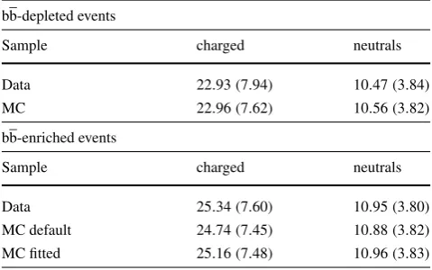
(PARU(44)) value set to 5.0 GeV/c. A first evaluation of the jet energies is obtained using the jets directions, energies, masses and imposing total energy-momentum conservation for the whole event. If the missing energy in a jet is larger than 1 GeV, a 4-vector is added to the jet. Its direction is taken to be the same as the jet direction and the missing mo-mentum is evaluated assuming that the missing particle mass is zero. Analysing simulated events, the relative uncertainty on the missing energy is measured to be 20%, and uncertain-ties on angles of the missing particle are 50 mrad. Energy momentum conservation is then applied again to the whole event, and particle parameters (for charged, neutral and pos-sibly missing) are fitted. After this procedure, 4-vectors of charged and neutral particles have been fitted, and possibly new 4-vectors corresponding to missing energy in each jet have been obtained. Jets are reevaluated (pjet) using this set of tracks and applying the same LUCLUS algorithm. Frac-tions of the fitted charged, neutral and missing energy are compared in Table4. Relative differences are at the level of a few 10−3. A comparison between data and the simula-tion has been also made for the averages and variances of charged and neutral particle multiplicities. The results are given in Table5.
Each jet pointing through the detector barrel region de-fined by|cosθjet|<0.75 is considered in turn, and charged particles belonging to the jet are used to reconstruct a B decay vertex candidate. It is then required that these tracks have at least two VD hits associated inRφand a minimum
Table 4 Fitted fractions of
charged energy(Ech.), neutral
energy(Eneu.)and their sum
reconstructed in bb-depleted and bb-enriched event samples in data and simulation. The missing energy(Emiss.)fitted
fraction is also given
bb-depleted events
Sample Ech.+Eneu. Ech. Eneu. Emiss.
Data 0.8644 0.5759 0.2879 0.1363
MC 0.8676 0.5778 0.2893 0.1323
(Data-MC)/MC −0.0037 −0.0033 −0.0048 +0.030
bb-enriched events
Sample Ech.+Eneu. Ech. Eneu. Emiss.
Data 0.8423 0.5891 0.2528 0.1589
MC 0.8423 0.5885 0.2535 0.1579
Table 5 Charged and neutral particle multiplicities (variances)
mea-sured in data and simulation
bb-depleted events
Sample charged neutrals
Data 22.93(7.94) 10.47(3.84) MC 22.96(7.62) 10.56(3.82)
bb-enriched events
Sample charged neutrals
Data 25.34(7.60) 10.95(3.80) MC default 24.74(7.45) 10.88(3.82) MC fitted 25.16(7.48) 10.96(3.83)
positive impact parameter with significance larger than√3σ relative to the main vertex of the event. A secondary vertex is then reconstructed. Tracks with a too large contribution to theχ2are removed from the fit in an iterative way. For a can-didate to be accepted, it is required that at least three tracks with theZ-coordinate measured in the VD remain, and that the distance between the secondary and the primary vertex projected along the jet direction is larger than 500 µm. The reconstructed mass must not exceed the B mass (all particles are assumed to be pions). If not, particles ordered by increas-ing values of their rapidity measured relative to the jet axis, are eliminated in turn. If the reconstructed mass is smaller than the B mass, particles belonging to the same jet ordered by decreasing rapidity values, are added in turn. For charged particles, offsets relative to the primary and secondary ver-tices are also examined. To possibly include a track, it is required that its offset relative to the secondary vertex is smaller than its offset relative to the primary vertex. The procedure is stopped when the mass of selected particles is closest to the B mass.
The B momentum is obtained by subtracting from the fit-ted jet momentum the momentum of the tracks from the jet, which have not been assigned to the B candidate. For the candidate to be accepted, the sum of the jet neutral energy
and of the charged energy for tracks that are simultaneously compatible with the primary and secondary vertices has to be smaller than 20 GeV. Figure3a shows the difference be-tween the reconstructed and the simulated B momentum, di-vided by the simulated value.
According to the simulation the applied algorithm has an average efficiency for the signal of 19% (see Fig.3b) and a contamination of 5% from non-b jets. The efficiency is rather flat forpweakB /pbeam>0.5 and is still 50% of its max-imum value aroundpweakB /pbeam=0.3. There are 134282 candidates selected in the data sample. The quoted efficiency for the signal differs from values given in Table3, because the latter refers to the whole event whereas the former is for b-jets after applying the additional cuts used in the analysis. Measured pBweak/pbeam distributions are compared in Fig.4with expectations from the simulation. The two distri-butions agree for bb-depleted events and show a marked dif-ference for events in the b-enriched sample. In what follows, the transformation of the non-perturbative QCD distribution used in the simulation, required to make the weighted dis-tribution of simulated events agree with the data, has been determined.
4.2.3 Determination of the b-hadron fragmentation distribution
The binned distribution of the reconstructedpBweak/pjet vari-able has been fitted by minimising aχ2, which includes ef-fects from the data and simulation statistics and from the weighting procedure.
In each bin the number of measured events is compared with an estimated number obtained in the following way: • contributions from background events are taken from the
qq simulation. They comprise three components: non-b jets in non-bb events, non-b jets in bb events and b jets from gluon splitting. In simulated events, the fractions of these components are respectively equal to 5.2%, 0.45% and 0.24% of the analysed events. The number of gluon splitting candidates has been multiplied by 1.5 to account for its measured rate at LEP [22].
Fig. 3 (a) distribution of
xp=(pBrec.−p gen.
B )/p gen.
B for weakly decaying b-hadrons. The full width at half maximum is equal to 16%. (b) acceptance for signal events versus
[image:13.595.50.290.75.225.2]Fig. 4 Comparison between the measured distributions of the beam
momentum fraction taken by a b-hadron, obtained in data (points
with error bars) and in the qq simulation (histogram). (a) Depleted
b-sample. (b) Enriched b-sample. The distributions have been nor-malised to unity
• The distribution of signal events is obtained by weighting bb simulated events. This weight contains several compo-nents, which have been determined to correct the values of parameters used in the simulation so that they agree with corresponding measured quantities as: B lifetimes, B charged particle multiplicity and B∗∗ fraction in jets. The used values of these measured quantities are the same as those used in the regularized unfolding analysis, as de-tailed in Sect.4.1.6.
• A weight, whose parameters are fitted, is also applied for each value of the simulatedzvariable (see Sect.2). The weights are constant over intervals inz(the weight func-tion is a histogram with a non-uniform binning).
• The normalisation of bb events is taken as a free parame-ter.
To prevent oscillations between the contents of nearby bins of the weight histogram, a regularisation term is in-cluded in theχ2:
χreg2 =C×2×n(i)−n(i−1)−n(i+1) 2, (9)
whereC is a parameter whose value (C=1) has been de-termined empirically using simulated events; andn(i)is the content of bini.
Distributions corrected for all effects are then obtained using corresponding generated distributions from simulated events before any selection criteria, and by applying the weight distribution fitted on real events, which depends on
thezvariable generated value for each simulated b-hadron. Statistical uncertainties in each bin, of these distributions, have been obtained using the full covariance matrix of the fitted parameters and generating toy experiments.
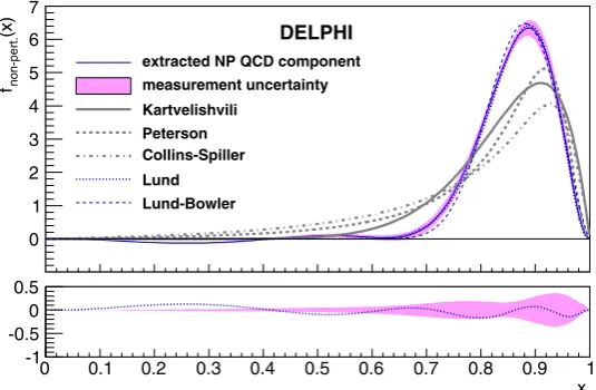
The fitted weight distribution obtained with the data sam-ple is given in Fig.5. This figure shows also thez distribu-tion as favoured by the data. It is rather different from the Peterson distribution which was used in the simulation, and shown on the same figure.
As in the companion analysis described in Sect.4.1, the differential b-quark fragmentation distribution is evaluated in nine intervals of thexBweakvariable whose averaged value is equal to xBweak =0.6978±0.0010. It is displayed in Fig.6. Measured values of the distribution in each bin and the corresponding statistical error matrix are given in Ap-pendixC. Its integral has been normalised to unity.
4.2.4 Systematic uncertainties
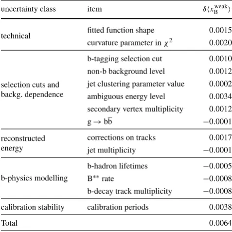
Systematic uncertainties have been evaluated for each value of the fragmentation distribution obtained in the ninexBweak intervals. In Table6, systematics onxBweakhave been re-ported. Sources of systematic uncertainties have been or-dered as in the previous analysis (Sect.4.1.6).
[image:14.595.306.543.415.642.2]Table 6 Systematic uncertainty on the mean value of thexBweak distri-bution in the weighted fitting analysis. The total is the sum in quadra-ture of all contributions. The sign indicates the correlation between the change in an uncertainty source and the shift in the final result. Uncer-tainties assigned by turning a weight on/off have no sign
uncertainty class item δxBweak
technical fitted function shape 0.0015 curvature parameter inχ2 0.0020
selection cuts and backg. dependence
b-tagging selection cut 0.0010 non-b background level 0.0012 jet clustering parameter value 0.0002 ambiguous energy level 0.0034 secondary vertex multiplicity 0.0012
g→bb −0.0001
reconstructed energy
corrections on tracks 0.0017 jet multiplicity −0.0001
b-physics modelling
b-hadron lifetimes −0.0005
B∗∗rate −0.0008
b-decay track multiplicity −0.0008
calibration stability calibration periods 0.0038
Total 0.0064
Technical systematics The weight function consists of twelve bins in zwhose content is fitted.6 Choices for the bin definition and bin number can induce a systematic un-certainty on the extracted distribution. This has been stud-ied by comparing the generated and fitted distributions in simulated events. Generated events correspond to the aver-age valuexweakB simgen..=0.7057 and have been reconstructed atxBweaksimrec..=0.7060. The quoted values have been cor-rected for the effect of the beam radiation which corresponds to an increase of 0.0015. The observed difference onxBweak is equal to+0.0003.
These results depend also on the choice for the value of the curvature parameterC introduced in theχ2 expression (see (9)). Changing the value of this parameter between 0.02 and 5.0 gives variations onxweakB at the level of ±0.002 on simulated events and even smaller values on real data events. In the following analysis the valueC=1 has been used and effects of the variation of this parameter between 0.02 and 5.0 are included in the evaluation of systematic uncertainties.
Selection cuts and background dependence In the analysed sample with the selectionPbtag≤10−3, the estimated frac-tion of non-b candidates amounts to 5.2%. In Table3it was
6The content of one of these bins is fixed to one as the normalisation of the signal bb events is also fitted.
observed that the fraction of selected events is a few % (rel-ative) higher in real data. As this effect remains in samples of high purity in bb events, its main origin comes most prob-ably from a difference in efficiency between real and sim-ulated bb events. A possible underestimate of the selection efficiency to non-bb events in the simulation amounts then to 10% (relative) at maximum. The effect of a±20% vari-ation on the non-b background level has been evaluated; it givesδxBweak = ±0.0012.
The stability of the measuredxBweakdistribution has been studied for different selections on the value of thePbtag vari-able. The resultingxBweakis stable within±0.001. For the corresponding systematic evaluation, half the difference ob-tained using selection cuts at 10−4and 10−10has been used. Hadronic jets have been reconstructed using the LU-CLUS algorithm with the value of the parameter defining the jets,djoin=5 GeV/c. Sensitivity of present results on the value of this parameter has been studied by redoing the mea-surements usingdjoin=10 GeV/c. The variation onxBweak is equal to+0.0002.
In a jet, there are charged particles which can be com-patible simultaneously with the primary and the secondary vertex. Concerning neutral particles, the angular resolution does not allow them to be attached with confidence to one of the two vertices. The energy taken by these two classes of tracks is denoted “ambiguous” energy. In the analysis, events have been selected requiring that the “ambiguous” energy is lower than 20 GeV. The stability of the results has been studied by changing the value for this selection crite-rion. A change from 20 GeV to 15 GeV results in a 25% decrease in the number of selected events, and no variation is measured forxBweak. A change from 15 GeV to 10 GeV keeps 50% of the initial statistics. The corresponding varia-tion is taken as a systematic uncertainty, which corresponds to a variation ofxBweakby−0.0034.
Events have been selected requiring at least three charged particles at the candidate B decay vertex. Taking the dif-ference observed for selections with at least three and five charged particles as an evaluation for the corresponding sys-tematic, the variation onxweakB is equal to+0.0012.
The rate for b-hadron production originating from gluon coupling to bb pairs has been measured by LEP experiments and found to be larger than the rate used in the simulation by a factor 1.5. The corresponding systematic uncertainty has been evaluated, considering the uncertainty, of 30%, ob-tained by DELPHI on this quantity [26]. The variation on xBweakis equal to−0.0001.
Reconstructed energy The analysis uses the beam energy as a constraint in a global fit of 4-momenta of charged and neutral particles, such that the total energy and momentum of the event is conserved.