Beta Stacy survival regression models

University of Warwick institutional repository: http://go.warwick.ac.uk/wrap

This paper is made available online in accordance with

publisher policies. Please scroll down to view the document

itself. Please refer to the repository record for this item and our

policy information available from the repository home page for

further information.

To see the final version of this paper please visit the publisher’s website

.

Access to the published version may require a subscription.

Author(s): F Rigat and P Muliere

Article Title: Beta-Stacy survival regression models

Year of publication: 2007

Link to published article:

http://www2.warwick.ac.uk/fac/sci/statistics/crism/research/2007/paper

07-6/

Beta-Stacy survival regression models

Fabio Rigat∗_{and Pietro Muliere}† April 11th 2007

Abstract

This paper introduces a class of survival models for discrete time-to-event data with random right censoring. Flexible distributions for the survival times are constructed by modelling the random survival func-tions as discrete-time beta-Stacy processes (DBS) and by introducing the regression effects via their prior means. Identifiability is attained by defining the DBS precision parameters as appropriate functions of the regression coefficients. By the conjugacy of the beta-Stacy process with respect to random right censoring, marginal posterior inferences for all model parameters can be efficiently approximated using the standard Gibbs sampler. The latter also yields a Monte Carlo approx-imation for the predictive distributions of the survival probabilities for future covariate profiles. We provide three clinical applications of the DBS survival regression framework comparing its estimates with those of parametric, semiparametric and non-parametric survival models.

Keywords: survival analysis, random right censoring, beta-Stacy pro-cess, Bayesian hierarchical models, Markov chain Monte Carlo, melanoma, cerebral palsy.

1

Introduction

This paper introduces a class of hierarchical regression models for discrete univariate time-to-event data with random right censoring. The distinc-tive feature of our approach is that the regression coefficients, the survival probabilities and their precision are represented by random parameters in-troduced via a hierarchical model structure. Our approach offers a flexible

∗_{(Corresponding author) CRiSM, Department of Statistics, University of Warwick,}

U.K.;email: [email protected]; tel: +44(0) 24 7657 5754; fax: +44(0)24 7652 4532

alternative to mixture modelling (Farewell [1982], Farewell [1986], Jewell [1982], Ibrahim et al. [2001]) and to semiparametric models (Cox [1972], Kalbfleisch [1978], Sinha and Dey [1996], Kleinman and Ibrahim [1998], Walker and Mallick [1999], Kottas and Gelfand [2001], De Blasi and Hjort [2007]). An advantage of the models presented here with respect to mixture models is that inference and prediction are carried out within a fixed param-eter space using the standard Gibbs sampler (Gelfand and Smith [1990]). Unlike the semiparametric proportional hazards model, the structure of our models is non-separable in the regression coefficients and in the random sur-vival processes. This assumption is relaxed by modelling the latter as a set of discrete time beta-Stacy processes (DBS) whose prior mean incorporates a regression component (Cifarelli et al. [1981]). The beta-Stacy process is a generalization of the Dirichlet process, in that more flexible prior beliefs are able to be represented and, unilke the Dirichlet process, is conjugate to right censored observations. Connections with beta process introduced by Hjort [1990] are immediate (Walker and Muliere [1997]). To ensure identifiability of the models thus constructed we define the DBS precision parameter so that large regression effects correspond to posterior survival processes con-centrated around their mean and vice versa. By the conjugacy of the DBS process the joint posterior distribution of our models’ parameters factors into the product of the prior distributions for the regression coefficients, the marginal likelihood of the survival data and the conditional posterior density of the survival probabilities. Similar results are obtained under a Dirichlet process prior in absence of censored observations in Mira and Petrone [1996], Dominici and Parmigiani [2001] and Carota and Parmigiani [2002], following Antoniak [1974] and Cifarelli and Regazzini [1978].

The hierarchical DBS framework is used in this paper to analyse clin-ical survival data recording the occurrence of events related to a patient’s status at discrete times such as days, weeks or months. In this context, the survival times can be thought of as taking values on a finite time grid of time points{τ1, . . . , τK} fixed by design. Under this assumption, each

indi-vidual’s survival distribution is a finite-dimensional random process defined by the random heights of its jumps at the grid points. We show that as long as all the observed survival times are included in the grid the posterior estimates are not sensitive to changes of its resolution.

and from the predictive distributions under a Weibull prior mean. Section 4.1 illustrates the analysis of the photocarcinogenic study of Grieve [1987] using both proportional hazards and accelerated failure time Weibull DBS models. The inferences obtained using the proportional hazards DBS model are compared with those of Dellaportas and Smith [1993] and with the non-parametric Kaplan-Meier (Kaplan and Meier [1958]) estimates. In Section 4.2 the Danish melanoma dataset of Andersen et al. [1993] is analysed. Un-like the Cox proportional hazards model (Cox [1972]), the DBS analysis of this dataset uncovers the significance of the skin resistance to the tumor infil-tration, the tumor thickness and the patients’ age at surgery as independent prognostic factors. Section 4.3 illustrates the results of a DBS analysis of the cerebral palsy survival data of Hutton and Pharoah [2002]. We confirm their findings with regard to the non-linear effect of birth weight on the sur-vival probability of the cerebral palsy patients. We also produce summaries of the predictive survival probabilities for the seven covariate profiles not included in the dataset. Should the next patient display one such covariate profiles, these predictions can be used for medical and legal purposes. Sec-tion 5 concludes the paper with a critical discussion of the DBS approach and by noting two possible generalizations.

2

The discrete beta-Stacy process

The beta-Stacy is a L´evy process introduced in Walker and Muliere [1997] as a non-parametric prior for the survival function of randomly right-censored survival times. Here we recall the constructive definition of its discrete-time version and we summarize its relevant properties for this work.

A scalar random variableY ∈(0, ) has a beta-Stacy distribution, with non-negative parameters (α, β, ), if its probability density function is

f(Y |α, β, ) = Γ(α+β) Γ(α)Γ(β)

Yα−1_(−Y)β−1

α+β−1 .

Its mean and variance are

E(Y | α, β, ) = α α+β

1 ,

V(Y | α, β, ) = αβ

(α+β)2_{(α+β+ 1)}

1 2.

IfY is beta-Stacy thenZ = Y

When each element of the orderedK-dimensional random vector{Yk}K

k=1

is conditionally independent beta-Stacy with parameters (αk, βk,1−Pj<kYj),

their joint distribution is generalized Dirichlet (Connor and Mosimann [1969]) with probability density function

fY(Y1, . . . , YK |α1, . . . , αk, β1, . . . , βK)∝ k

Y

k=1

Yαk−1

k

(1−P

j≤kYj)βk−1

(1−P

j<kYj)αk+βk−1

. (1)

The standard Dirichlet density obtains ifβk−1 =βk+αk for k= 1, ..., K.

If {Yk}K_k=1 is jointly generalised Dirichlet and Sk = 1−Pj≤kYj, then {Sk}K_k=1is a discrete-time beta-Stacy process (DBS) with parameters{αk, βk}Kk=1,

written as

{Sk}Kk=1 ∼ DBS {αk, βk}Kk=1

.

In what follows the DBS process is used as the prior distribution for the survival probabilities {Sk}Kk=1 having random jumps {Yk}Kk=1 at the fixed

time pointsτ ={τ₁, . . . , τK}. Let t = {ti}N

i=1 and δ = {δi}Ni=1 represent a sample of univariate

ran-dom survival times with δi = 1 if ti is observed exactly and δi = 0 if

ti is right-censored at random. Let τ be such that Pk1{ti=τk} = 1 for

i = 1, . . . , N. If the survival probabilities of each individual are a priori

{Si,k}Kk=1 ∼ DBS({αi,k, βi,k}Kk=1), by Theorem 1 of Walker and Muliere

[1997] their posterior distributions are

{Si,k}K_k=1|ti, δi∼ DBS {αi,k+ni,k, βi,k+mi,k}Kk=1

,

with

ni,k = 1{ti=τk,δi=1},

mi,k = 1{ti≥τk,δi=0}+ 1{ti>τk,δi=1}.

The conjugacy of the beta-Stacy process with respect to random right cen-soring also yields a closed form expression for their marginal posterior pre-dictive survival probabilities, that is

p(tN+1 =τk|ti, δi,{αi,j, βi,j}kj=1) =

αi,k+ni,k

αi,k+βi,k+ni,k+mi,k

Q

j<k

βi,j+mi,j

αi,j+βi,j+ni,j+mi,j.

2.1 Marginal likelihood for DBS survival models

To construct a class of survival regression models using the discrete DBS process prior, we follow Walker and Muliere [1997] by letting{αi,k, βi,k} be

αi,k = νi(Gi,k−Gi,k−1), (2)

for i = 1, . . . , N and k = 1, . . . , K. Here Gi,k represents the prior mean

cumulative distribution function (CDF) at time τk for the survival time of

individualiand the coefficientνi≥0 represents their prior precision. When

the DBS parameters are defined as in (2) and (3) we write

{Si,k}Kk=1∼ DBS νi,{Gi,k}Kk=1

.

Under this parametrization the prior mean and variance of the increments of the survival functionYi,k= (Si,k−Si,k−1) =P(ti=τk) are (Connor and

Mosimann [1969])

E(Yi,k|Gi,k, Gi,k−1) =Gi,k−Gi,k−1, (4)

V(Yi,k|νi,{Gi,j}kj=1) = (Gi,k−Gi,k−1)×

×1+νi(Gi,k−Gi,k−1)

νi(1−Gi,k−1)+1

Q

j<k

1+νi(1−Gi,j)

1+νi(1−Gi,j−1)−(Gi,k−Gi,k−1)

, (5)

and forl < k their covariance is

Cov(Yi,l, Yi,k|νi,{Gi,j}kj=1) = (Gi,k−Gi,k−1)×

×1+νi(Gi,l−Gi,l−1)

νi(1−Gi,l−1)+1

Q

j<l

1+νi(1−Gi,j)

1+νi(1−Gi,j−1)−(Gi,l−Gi,l−1)

.

By equation (4) the prior survival probability for individual iat time τk is

centered around its prior mean (1−Gi,k). The right-hand side of equation

(5) is decreasing in νi, which motivates the interpretation of the latter as

the prior precision for the survival probabilities. By (2) and (3) we have αi,k+βi,k =βi,k−1, so that the survival probabilities for each individual are

assigned a discrete Dirichlet process prior and have a discrete beta-Stacy posterior. Within this framework the prior coefficientνi can be interpreted

as a measure of the prior strenght of belief in modelGi,k (Ferguson [1974],

Antoniak [1974], Ferguson and Phadia [1979], Kuo [1983], Brunner and Lo [1989], Muliere and Tardella [1998], Escobar [1994]).

Let G = {{Gi,k}Kk=1}Ni=1 be a N ×K matrix including the prior mean

CDF values for all samples atτ. The marginal probability mass function of the survival times is

p(t|δ,G, τ) =Q

i,k

_(G

i,k−Gi,k−1)δi(1−Gi,k)1−δi

(1−Gi,k−1)

Q

j<k

(1−Gi,j)

(1−Gi,j−1)

1{_ti=_τk}

.(6)

Equation (6) is derived in the Appendix. The analogy between (6) and parametric models which do not allow for the randomness of the survival function itself can be seen when τ1 = 0 and τk−τk−1 = ∆K = _K1 for all

to Lebesgue measure, if K → ∞ the right-hand side of (6) approximates the likelihood function of the conditionally independent right-censored data tunder model G(·).

3

Hierarchical DBS regression models

When the covariate profilesXi = [Xi,1, . . . , Xi,q] are given for each sample

uniti= 1, . . . , N, a regression component is incorporated in the prior mean modelG(·) by letting

Gi,k(Xi, θ, η) =G(ti≤τk|Xi, θ, η),

whereθ represents a q×1 vector or regression effects and η are additional parameters indexing the prior mean CDF. We propose constructing flexible survival models by letting the distribution of the survival datati at the time

pointsτ be represented by the DBS random survival probabilities{Si,k}K

k=1

centered around their mean survival function 1−Gi,k(Xi, θ, η) with

preci-sion νi. However, if both the coefficients (θ, η) indexing G(·) and the DBS

precision parameters (ν₁, ..., νN) are unknown, such models are not

identi-fiable from the data. This can be seen by considering that under (2) and (3) the generalised Dirichlet density for the survival probabilities of individ-ual i may not be integrable with respect to νi. The same issue has been

noted by Dominici and Parmigiani [2001] and by Carota and Parmigiani [2002] with regard to the total mass parameter of their Dirichlet process priors. In this paper we identify the hierarchical DBS models by defining the covariate-specific precisions as

νi= (Xiθ)2. (7)

By (7) when the regression coefficients are large in absolute value the DBS random survival probabilities are concentrated around their mean and vice versa. Therefore, under (7) the random survival probabilities have a promi-nent role to fit the survival data only when their relationship with the co-variates is weak under modelG(·).

The hierarchy of the DBS survival regression models is completed by the specification of the prior distributions for the coefficients (θ, η). By letting S = {{Si,k}K

k=1}Ni=1 and by assuming that the survival times t are

the hierarchy can be written as

(θ, η)∼fθ,η(θ, η),

{Si,k}Kk=1 ∼ DBS (Xiθ)2,{G(ti ≤τk|Xi, θ, η)}Kk=1

fori= 1, . . . , N,

P(t| δ,S, τ) =Q

i,k

(Si,k−1−Si,k)δiS_i,k1−δi

1_{ti=_τk}

, (8)

withSi,0 = 1 for alli= 1, ..., N. We adopt two alternative formulations for

the regression component under a Weibull prior mean survival functionG, namely

GP H(t≤τ |Xθ, η) = 1−e−e

Xθ_τη

, (9)

GAF T(t≤τ |Xθ, η) = 1−e−(e

Xθ_τ)η

, (10)

whereX is theN×qmatrix whichith rowXirepresents the covariate profile

for individuali. Here the Weibull distribution is adopted for the availability of a closed form expression for the survival function 1−G(·). Equation (9) assumes that the prior mean cumulative hazard processess for individuals having different covariate profiles are proportional at different time points (Cox [1972]). Equation (10) adopts an accelerated failure time regression (Prentice and Kalbfleisch [1979]) where the survival time is shifted along the time axis proportionally to a stress factor. The latter is represented by the exponential of the linear predictor Xθ as in Walker and Mallick [1999]. The coefficient η in (9) and in (10) is the Weibull index parameter, which determines the convexity of the prior mean survival distribution for all individuals over time.

3.1 Parameter estimation

Under (9) and (10) the unknown parameters of the DBS survival models are (θ, η,S). A key feature of (8) is that the joint posterior density factors as

f(θ, η,S |t, δ, X) =f(θ, η)p(t|δ,G(Xθ, η), τ)fS(S| t, δ,G(Xθ, η)),(11)

whereG(Xθ, η) ={{Gi,k(Xiθ, η)}Kk=1}Ni=1,p(t|δ,G(Xθ, η), τ) is the marginal

likelihood of the survival data (6),f(θ, η) represents the joint prior density for (θ, η) andfS(S|t, δ,G(Xθ, η)) is the product of the generalized Dirichlet

of a closed-form expression for the marginal likelihood of the data condi-tionally on the parameters of their random distributions. In previous works the marginal likelihood for exact data is obtained using a Dirichlet process prior whereas in this work equation (6) was derived for discrete randomly right-censored survival times using the conjugacy of the DBS process.

In what follows we let the priors for the coefficients θ and η be respec-tively Gaussian N(m, s) with fixed mean m and standard deviation s and gammaGa(a_b2,b_a), having mean aand variance b. To elicit the prior hyper parameters (m, s, a, b) we consider the corresponding marginal prior pre-dictive survival processes. Since the generalised Dirichlet density cannot be marginalised analytically with respect to the priors for (θ, η) we use a Monte Carlo strategy. For given values of (m, s, a, b) we sample an array of realisations of (θ, η) from their priors and we generate corresponding realisa-tions of the DBS prior survival processes for each distinct covariate profile. The sample distribution of the generated survival probabilities approximates their marginal prior distribution, thus representing the marginal effect of a given configuration (m, s, a, b) on the prior predictive survival functions. In what follows a set of values for (m, s, a, b) is adopted if the corresponding prior predictive mean survival probabilities atτ and their 95% prior proba-bility intervals are considered appropriate for the data to be analysed.

The conditional posterior densities for (θ, η) are log-concave but they are not available for exact sampling, so that approximate marginal posterior in-ferences can be computed via the Gibbs sampler (Gelfand and Smith [1990], Tierney [1998]) using a Metropolis-Hastings (MH) rejection step (Hastings [1970]). The posterior inferences reported in Section 4 were computed using a component-wise random walk MH update for (θ, η). For each component of θ we employ a Gaussian proposal density centerd at its current value whereas for the Weibull indexη we use a gamma random walk proposal of the form Ga(η2w

Cη,

Cη

ηw) where ηw represents the current value of η and Cη is a fixed coefficient. Under this parametrization the proposal mean isηw and

its variance isCη. The survival probabilitiesS are updated exactly within

the Gibbs sampler using the constructive definition of the DBS process of Section 2. When the covariate profiles of all N samples are distinct, the parameters of their generalized Dirichlet conditional posterior densities are

α∗_i,k = (Xiθ)2(Gi,k(Xiθ, η)−Gi,k−1(Xiθ, η)) +δi1{ti=τk},

β_i,k∗ = (Xiθ)2(1−Gi,k(Xiθ, η)) +δi1{ti>τk}+ 1{ti≥τk,δi=0}.

let{g(i)}N

i=1 be the group label of theith observation, with 1≤g(i)≤N for

all values ofi. The posterior parameters of the DBS process for the survival probabilities for group g(i) are

α∗_g(i),k = (X_g(i)θ)2 Gi,k(Xg(i)θ, η)−Gi,k−1(Xg(i)θ, η)

+ X

i=g(i)

δi1{ti=τk},(12)

β_g∗_(i),k = (Xg(i)θ)2 1−Gi,k(Xg(i)θ, η)

+ X

i=g(i)

δi1{ti>τk}+ 1{ti≥τk,δi=0}.(13)

3.2 Predictions

LettN+1 be the unknown exact survival time for a future sample with

co-variatesX_g(N+1). According to the hierarchy (8), ifX_g(N+1) =Xi∗ for some

i∗ ∈[1, N], the distribution of the survival probabilities (SN+1,1, ..., SN+1,K)

coincides with that of (Si∗_,1, ..., S_i∗_,K), so that summaries of their Gibbs

sampler draws provide approximate marginal posterior predictions fortN+1

at the time pointsτ. When X_g(N+1) does not coincide with any of the ob-served covariate profiles, approximate marginal posterior predictions can be computed using the Gibbs sampler draws{θw, ηw}Mw=1. For instance, within

the DBS framework the marginal posterior predictions for the survival time of patient (N + 1) with covariates Xg(N+1) at time τk are summaries of

the random variable SN+1,k given (t, δ, X, Xg(N+1)). Its conditional

pos-terior distribution can be sampled exactly by drawing a realization of the increments (SN+1,1, SN+1,2−SN+1,1, ..., SN+1,k−SN+1,k−1) for each couple

(θw, ηw) using their generalised Dirichlet joint posterior distribution.

Sum-maries of the sequence {SN+1,k(w)}Mw=B+1 thus generated provide a Monte

Carlo approximation of its marginal posterior moments. These summaries can be used to evaluate the survival perspective of a future patient which clinical profile X_g(N+1) has not been observed in the past. If X_g(N+1) in-cludes covariates which value can be controlled, such as treatments, esti-mates ofSN+1,k under alternative scenarios indicate which combinations of

values ofX_g(N+1) correspond to the highest survival rates at timeτkhaving

observed (t, δ, X).

4

Applications of the model

4.1 Analysis of the mice dataset

photocarcinogenic treatment to assess whether pre-treatment with a test substance (8-MOP) shortens the time to occurrence of skin tumors (Grieve [1987]). This data have been analysed via a proportional hazards Weibull survival model by Grieve [1987] using the numerical integration techniques of Naylor and Smith [1982] and by Dellaportas and Smith [1993], who fitted the same model using the Gibbs sampler. In this Section we analyse the mice data via the DBS Weibull survival models using the PH and AFT regressions (9) and (10) under two specifications of the time grid τ. The latter include respectively the months (1, ...,40) and all time points between 1 and 40 months equally spaced by 0.1 months. The first specification of τ matches the resolution and range of the survival data, which facilitates the comparison between the DBS estimates of the survival probabilities and the nonparametric Kaplan-Meier (KM; Kaplan and Meier [1958]) estimates. The second time grid represents a ten-fold increase in the number of time points over the same range. The comparison of the posterior estimates for the two specifications of τ informs on the sensitivity of the posterior distributions of (θ, η,S) with respect to the resolution of the time grid. Posterior sampling was carried out for fifty thousand iterations via the Gibbs sampler described in Section 3. All posterior estimates were computed using the last twenty five thousand samples.

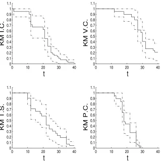
Figure 1 shows the KM estimates of the survival curves for the four groups along with their 95% point-wise confidence intervals. The estimated group medians in months are respectively 21(13,23) for group 1 (irradi-ated controls), 22(15,26) for group 2 (test substance: 8-methoxypsoralen), 18(17,22) for group 3 (positive controls) and 30(27,32) for group 4 (vehicle controls), implying that the survival perspective for the mice belonging to the vehicle control group is better that those of the other groups.

0 10 20 30 40 0 0.1 0.2 0.3 0.4 0.5 0.6 0.7 0.8 0.9 1 1.1

t

0 10 20 30 40 0 0.1 0.2 0.3 0.4 0.5 0.6 0.7 0.8 0.9 1 1.1

t

0 10 20 30 40 0 0.1 0.2 0.3 0.4 0.5 0.6 0.7 0.8 0.9 1 1.1

t

0 10 20 30 40 0 0.1 0.2 0.3 0.4 0.5 0.6 0.7 0.8 0.9 1 1.1

t

Figure 1: Kaplan-Meier estimates of the survival probabilities for the four groups composing the mice dataset (I.C. = irradiated control, T.S. = test substance (8-MOP), P.C. = positive control, V.C. = vehicle control). Their 95% confidence intervals were computed using Greenwood’s formula. The estimates show that the survival perspective for the mice belonging to the vehicle control group is better that those of the other groups.

for (m, s, a, b), which allows an average 10−15% of all mice to survive until month 40 irrespectively of their treatment.

left-0 5 10 15 20 25 30 35 40 0 0.1 0.2 0.3 0.4 0.5 0.6 0.7 0.8 0.9 1 τ

Prior pred. S(

τ

) (PH)

0 5 10 15 20 25 30 35 40 0 0.1 0.2 0.3 0.4 0.5 0.6 0.7 0.8 0.9 1 τ

Prior pred. S(

τ

) (AFT)

0 5 10 15 20 25 30 35 40 0 0.1 0.2 0.3 0.4 0.5 0.6 0.7 0.8 0.9 1 τ

Prior pred. S(

τ

) (PH)

0 5 10 15 20 25 30 35 40 0 0.1 0.2 0.3 0.4 0.5 0.6 0.7 0.8 0.9 1 τ

Prior pred. S(

τ

) (AFT)

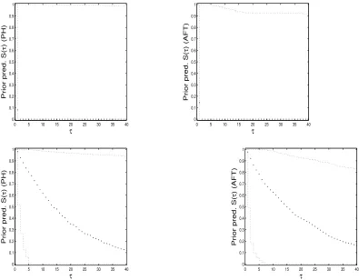
Figure 2: prior predictive sample mean survival probabilities and their 95% prior predictive HPDs under two alternative values of the prior hyper-parameters for (θ, η) (respectively m = 0, s = 1, a= 1, b = 1 in the first row and m = −2, s = 1, a= 1, b= 0.1 in the second row). The prior predictive summaries were computed using samples of size 10000 from the marginal priors for (θ, η). The second prior setting was adopted for the DBS analysis of the mice data.

respect to those of the other three groups, implying that the survival prob-abilities of the individuals belonging to group 4 are higher than those of the other groups. This conclusion is consistent with the KM estimates shows in Figure 1. The large overlapping between the estimated 95% posterior intervals reported in Tables 1 and 2 suggests that the higher resoultion of the time gridτ does not affect significantly the posterior estimates of (θ, η). Figures 3 through 6 illustrate the posterior estimates of the survival

proba-P H P H10 DS

θI.C. −4.65(−5.41,−3.96) −4.46(−5.24,−3.77) −4.63(−5.41,−3.84)

θT.S. −4.90(−5.77,−4.09) −4.66(−5.43,−3.90) −4.86(−5.69,−4.04)

θP.C. −4.60(−5.33,−3.89) −4.40(−5.20,−3.95) −4.60(−5.37,−3.80)

θV.C. −5.42(−6.22,−4.60) −5.17(−6.10,−4.45) −5.37(−6.26,−4.53)

η 1.47(1.26,1.68) 1.40(1.21,1.60) 1.92(1.41,2.44) I.C. 23(16,27) 22(16,27) 18.75(13.95,25.13) T.S. 24(18,30) 24(17.6,31) 21.95(16.04,30.13) P.C. 21(17,26) 20.6(17,26) 18.15(13.26,24.81) V.C. 32(27,40) 32(27,40) 31.47(22.41,44.50)

Table 1: posterior estimates of (θ, η) and posterior predictive median survival times obtained using the DBS model with PH regression and the DS model. The esti-mated regression coefficientθV.C. is lower than the estimates of the other groups, implying that the posterior mean survival probabilities of the individuals belonging to the vehicle control group are higher than those of the other groups.

AF T AF T10

θI.C. −3.25(−3.46,−3.05) −3.26(−3.47,−3.08)

θT.S. −3.38(−3.62,−3.17) −3.39(−3.62,−3.19)

θP.C. −3.15(−3.37,−2.95) −3.18(−3.40,−2.98)

θV.C. −3.69(−3.93,−2.95) −3.70(−3.94,−3.48)

η 2.92(1.85,2.78) 2.33(1.87,2.83) I.C. 23(20,27) 23(20,27.2) T.S. 26(19,32) 26(19.3,31)

P.C. 22(18,26) 22(18,26)

V.C. 32(28,40) 32(28.1,40)

Table 2: posterior estimates of (θ, η) and posterior predictive median survival times obtained using the DBS model with AFT regression. Consistently with the esti-mates of the PH model, the AFT model confirms that the mean mortality of the vehicle control group is the lowest.

their covariate-dependent Weibull centering distribution.

4.2 Analysis of the Danish mealanoma survival data

0 10 20 30 40 0 0.1 0.2 0.3 0.4 0.5 0.6 0.7 0.8 0.9 1 1.1

τ

0 10 20 30 40 0 0.1 0.2 0.3 0.4 0.5 0.6 0.7 0.8 0.9 1 1.1

τ

0 10 20 30 40 0 0.1 0.2 0.3 0.4 0.5 0.6 0.7 0.8 0.9 1 1.1

τ

0 10 20 30 40 0 0.1 0.2 0.3 0.4 0.5 0.6 0.7 0.8 0.9 1 1.1

τ

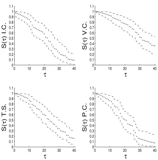
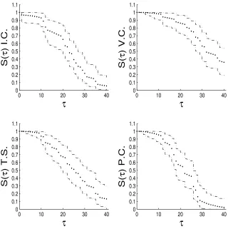
Figure 3: posterior estimates for the DBS survival probabilities for the four mice groups under PH regression and coarser time grid.

0 10 20 30 40 0 0.1 0.2 0.3 0.4 0.5 0.6 0.7 0.8 0.9 1 1.1

τ

0 10 20 30 40 0 0.1 0.2 0.3 0.4 0.5 0.6 0.7 0.8 0.9 1 1.1

τ

0 10 20 30 40 0 0.1 0.2 0.3 0.4 0.5 0.6 0.7 0.8 0.9 1 1.1

τ

0 10 20 30 40 0 0.1 0.2 0.3 0.4 0.5 0.6 0.7 0.8 0.9 1 1.1

τ

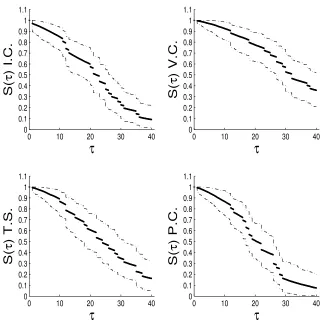
Figure 4: posterior estimates for the DBS survival probabilities for the four mice groups under PH regression and finer time grid.

0 10 20 30 40 0 0.1 0.2 0.3 0.4 0.5 0.6 0.7 0.8 0.9 1 1.1

τ

0 10 20 30 40 0 0.1 0.2 0.3 0.4 0.5 0.6 0.7 0.8 0.9 1 1.1

τ

0 10 20 30 40 0 0.1 0.2 0.3 0.4 0.5 0.6 0.7 0.8 0.9 1 1.1

τ

0 10 20 30 40 0 0.1 0.2 0.3 0.4 0.5 0.6 0.7 0.8 0.9 1 1.1

τ

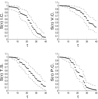
Figure 5: posterior estimates for the DBS survival probabilities for the four mice groups under AFT regression and coarser time grid.

distribution for the prior predictive medians for the survival times of all individuals over the range of the data ((0,183) months).

0 10 20 30 40 0 0.1 0.2 0.3 0.4 0.5 0.6 0.7 0.8 0.9 1 1.1

τ

0 10 20 30 40 0 0.1 0.2 0.3 0.4 0.5 0.6 0.7 0.8 0.9 1 1.1

τ

0 10 20 30 40 0 0.1 0.2 0.3 0.4 0.5 0.6 0.7 0.8 0.9 1 1.1

τ

0 10 20 30 40 0 0.1 0.2 0.3 0.4 0.5 0.6 0.7 0.8 0.9 1 1.1

τ

Figure 6: posterior estimates for the DBS survival probabilities for the four mice groups under AFT regression and finer time grid.

data groups may not be proportional, as pointed out in Andersen et al. [1993].

patients are young females presenting uninfiltrated thick melanomas with-out epithelioid cells. The predictive survival probabilities are higher for pa-tients displaying deep tumors with respect to cases of superficial melanomas. The highest median survival at five years after surgery correspond to deep melanomas with or without skin ulceration (respectively 0.65(0.43,0.97) and 0.87(0.50,0.99)) whereas the lowest estimated survival probabilities corre-spond to superficial tumors with or without skin ulceration (respectively 0.03(0.01,0.10) and 0.06(0.02,0.22)).

Coefficient DBS post. est. Cox PH

θdepth −0.44(−0.92,−0.01) −0.54(−1.03,−0.05)

θresistance −1.16(−1.53,−0.78) −0.01(−0.35,0.35)

θepithelioid −1.14(−1.55,−0.75) −0.16(−0.52,0.19)

θulceration 0.10(−0.35,0.53) 0.06(−0.30,0.43)

θthick 0.61(0.06,1.15) 0.87(−0.36,1.38)

θmale −0.75(−1.20,−0.34) −0.08(−0.44,0.28)

θage −0.91(−1.36,−0.53) −0.79(−1.15,−0.42)

η 0.22(0.18,0.26)

-Table 3: DBS posterior estimates of (θ, η) for the melanoma survival data under the PH regression and the Cox semiparametric survival regression model. According to the DBS estimates all covariates but the ulceration status are significant predictors of the survival time, whereas only the tumor depth and the patients’ age are found significant by the Cox model.

4.3 Cerebral palsy survival times

0 50 100 150 200 0

0.1 0.2 0.3 0.4 0.5 0.6 0.7 0.8 0.9 1

τ

Predictive S(

τ

)

Figure 7: estimated marginal posterior predictive median survival probabilities at five years from surgery for four hypothetical future patients whose covari-ate profiles are not included among the 201 melanoma patients. The four pa-tients are young females presenting uninfiltrated thick melanomas without ep-ithelioid cells. The highest median survival probabilities correspond to deep melanomas with (0.65(0.43,0.97)) or without (0.87(0.50,0.99)) skin ulceration whereas the lowest estimated survival probabilities correspond to superficial tu-mors with (0.03(0.01,0.10)) or without (0.06(0.02,0.22)) skin ulceration.

effects of birth weight found by Hutton and Pharoah [2002] this predictor was categorized in three classes, based on its 33rd and 66th percentiles, which are: [580,2264), [2264,3147) and [3147,5260) grams. The prior for the regression parametersθand for the Weibull indexηare respectivelyN(−1,1) and Ga(1,0.1). As in the previous example, these priors correspond to approximately uniformly distributed prior predictive median survival times over the range of the observed survival times. Posterior sampling was carried out for twenty five thousand iterations using the Gibbs sampler described in Section 3. Posterior estimates and predictions were computed using the last ten thousand iterations.

sur-vival probabilities for individuals with weight at birth between [3147,5260) grams is the lowest whereas those of individuals with birth weight between [580,2264) grams is the highest. The difference between estimates of the birth weight categories indicate a non-linear effect on the mean survival probabilities consistenly with the results of Hutton and Pharoah [2002]. The estimated Weibull index parameter η indicates that an exponential mean model is adequate for this dataset. Figure 8 displays the posterior

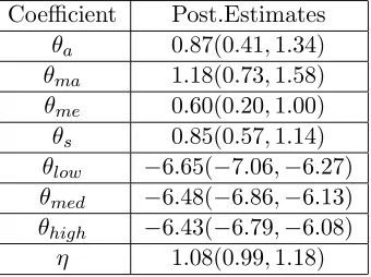
Coefficient Post.Estimates θa 0.87(0.41,1.34)

θma 1.18(0.73,1.58)

θme 0.60(0.20,1.00)

θs 0.85(0.57,1.14)

θlow −6.65(−7.06,−6.27)

θmed −6.48(−6.86,−6.13)

θhigh −6.43(−6.79,−6.08)

η 1.08(0.99,1.18)

Table 4: posterior estimates of the regression parameters and for the Weibull index for the cerebral palsy dataset. The occurrence of any impairment worsens the survival perspective, with manual impairment being the most severe. The effect of the birth weight on the mean survival probabilities appears to be non-linear. All other factors being constant, individuals with low birth weight ([580,2264) grams) have the best survival whereas those with high birth weight ([3147,5260) grams) have the worse perspective.

mean survival probabilities and their 95% posterior intervals for the best and the worst case in the dataset. The latter displays ambulatory, manual and mental impairments and has medium birth weigth whereas the former does not present any impairment at the same birth weight.

0 5 10 15 20 25 30 35 40 45 0

0.1 0.2 0.3 0.4 0.5 0.6 0.7 0.8 0.9 1

τ

Post. mean S(

τ

)

Figure 8: best and worst estimated survival probabilities among the 1585 cerabral palsy patients. The central dots represent the estimated posterior mean survival probabilities at the grid pointsτ. The dashed lines represent the survival probabil-ities’ estimated 95% posterior intervals. The worse survival prespective is associ-ated to ambulatory, manual and mental impairments and has medium birth weigth whereas the covariate profile corresponding to the best survival does not present any impairment at the same birth weight.

is due to admitted medical malpractice, these predictions can provide a ref-erence to determine the quantum of a compensation based on the child’s survival probabilities. The highest predicted survival corresponds to future individuals having ambulatory impairment only and birth weight within [3147,5260) grams, whereas the worse predictions correspond to individuals within the same birth weight categoty and displaying manual, mental and sight impairments.

5

Discussion

Profile Est. S(24.5) a, [3147,5260)gr 0.90(0.73,0.98) a,s, [580,2264)gr 0.74(0.46,0.93) a,s, [3147,5260)gr 0.69(0.41,0.89) ma,s, [580,2264)gr 0.68(0.36,0.88) ma,s, [2264,3147)gr 0.62(0.29,0.86) ma,me,s, [580,2264)gr 0.38(0.08,0.70) ma,me,s, [3147,5260)gr 0.29(0.03,0.66)

Table 5: posterior predictive median survival probabilities at 24.5 years from birth and end-points of their 95% HPDs for the 7 profiles for which no observation is available. The highest predicted survival corresponds to future individuals having ambulatory impairment only and birth weight within [3147,5260) grams, whereas the worse predictions correspond to individuals within the same birth weight cate-goty and with manual, mental and sight impairments.

time and covariate dependent frailty parameters conferring flexibility to the survival processes.

The DBS framework represents an intermediate modelling framework between parametric and non-parametric survival models. While sharing with the former an interpretable parameter structure, the number of DBS random survival probabilities can be large as it is typically the case for semi-parametric and non-semi-parametric models. Having a potentially large number of unknown parameters is not computationally cumbersome in our work because, by the conjugacy of the discrete beta-Stacy process, all survival probabilities are updated exactly in one step within the Gibbs sampler.

linear predictor.

The example of Section 4.1 shows that the posterior estimates of the survival probabilities and those of the regession parameters are consistent with those of Dellaportas and Smith [1993] and with the non-parametric Kaplan-Meier estimates. The posterior estimates are also found to be not significantly affected by the resolution ofτ as long as all the observed sur-vival times are included. The examples of Sections 4.2 and 4.3 demonstrate the relevance of the DBS framework for clinical applications. The results presented in Section 4.2 support those of Andersen et al. [1993] and the re-cent directives included in the American Joint Committee on Cancer Staging Manual, empsasizing the key role of the tumor thickness, the skin resistance to tumor infiltration and the patients’ age at surgery as independent prog-nostic factors of survival. The analysis of the cerebral palsy data of Section 4.3 confirms a non-linear effect of the birth weight on survival and it provides flexible predictions for the survival times associated to the seven covariate profiles not included in the dataset.

Throughout this paper we let the resolution of τ be fixed by design. When the position of some of the time points ofτ cannot be fixed in advance, since the beta-Stacy is a L´evy process the algorithms of Walker and Damien [1998] and Wolpert and Ickstadt [1998] can be used to efficiently generate draws from their conditional posterior distributions. If also the number of jumps needs to be a priori unknown, a reversible jump step (Green [1995]) can be added to their samplers.

A second generalization of the DBS paradigm beyond the scope of this work allows for the covariate-dependent grouping structure of the different samples{g(i)}N

i=1to be a priori unknown. In the current model formulation,

different individuals share a common survival process only if their covariate profiles are identical. However, when their covariate profiles are similar it might be possible to associate to all such individuals a common survival pro-cess. This extension of the DBS paradigm can thus lead to the construction of more parsimonious models when the covariate profiles of several groups of individuals are similar among themselves.

Appendix

α = {{αi,k}N

i=1}Kk=1, β ={{βi,k}Ni=1}Kk=1 and Si ={Si,k}K_k=1. By assuming

that the survival times of the N samples are independent conditionally on their survival probabilities, this integral can be written as

p(t|δ, τ, α, β) =QN

i=1 R Si QK k=1

(Si,k−1−Si,k)δiSi,k1−δi

1{_ti=_τk} ×

× Γ(αi,k+βi,k)

Γ(αi,k)Γ(βi,k)(Si,k−1−Si,k)

αi,k−1 S

βi,k−1 i,k

S_i,kαi,k₋+₁βi,k−1dSi.

Let nowYi,k=Si,k−1−Si,kandYi={Yi,k}Kk=1. As shown in Section 2, if the

joint prior for the survival probabilities Si is a discrete beta-Stacy process,

it follows thatYi,kis conditionally distributed asBS(αi,k, βi,k,1−Pj<kYi,j)

and vice versa. Therefore, the integral can be rewritten as a function of the random jumps of the survival functionY as

p(t|δ, τ, α, β) =QN

i=1 R Yi QK k=1

Yδi

i,k(1−

P

j≤kYi,j)1−δi

1_{ti=_τk} ×

× Γ(αi,k+βi,k)

Γ(αi,k)Γ(βi,k)Y

αi,k−1

i,k

(1−P

j≤kYi,j)βi,k−1

(1−P

j<kYi,j)αi,k+βi,k−1

dYi. (14)

The K-dimensional integral on the right-hand side of equation (14) can be solved with respect to each of its coordinatesYi,kin turn, starting fromYi,K.

The expression of the marginal likelihood (6) follows by observing that

E(Yi,k|αi,k, βi,k, δi) =

αδi

i,kβ

1−δi

i,k

αi,k+βi,k

Y

j<k

βi,j

αi,j+βi,j

,

and by substituting the expressions for the beta-Stacy hyperparameters (2) and (3).

Acknowledgements

References

P.K. Andersen, O. Borgan, R.D. Gill, and N. Keiding. Statistical Models Based on Counting Processes. Springer, 1993.

C. Antoniak. Mixtures of Dirichlet processes with applications to Bayesian Non-parametric problems. The Annals of Statistics, 2:1152–1174, 1974.

L.Y. Brunner and A.Y. Lo. Bayes methods for a symmetric unimodal density and its mode. The Annals of Statistics, 17:1550–1566, 1989.

C. Carota and G. Parmigiani. Semiparametric regression for count data.

Biometrika, 89:265–281, 2002.

D.M. Cifarelli and E. Regazzini. Problemi statistici non parametrici in condizioni di scambiabilita’parziale. Impiego di medie associative. Quaderni dell’Istituto di Matematica Finanziaria dell’Universita’di Torino, III, 12:1–36, 1978.

D.M. Cifarelli, P. Muliere, and M. Scarsini. Il modello lineare nell’approccio Bayesiano non parametrico. Technical Report, Istituto Matematico G. Castel-nuovo, Universit´a di Roma, 1981.

R.J. Connor and J.E. Mosimann. Concepts of independence for proportions with a generalization of the Dirichlet distribution. Journal of the American Statistical Association, 64:194–206, 1969.

D.R. Cox. Regression models and life tables.Journal of the Royal Statistical Society Series B, 34:187–220, 1972.

P. De Blasi and N.L. Hjort. Bayesian survival analysis in proportional hazard models with logistic relative risk. Scandinavial Journal of Statistics, 34:229–257, 2007.

P. Dellaportas and A.F.M. Smith. Bayesian inference for Generalised Linear and Proportional Hazards models via Gibbs sampling.Applied Statistics, 42:443–459, 1993.

F. Dominici and G. Parmigiani. Bayesian semiparametric analysis of developmental toxicology data. Biometrics, 57:150–157, 2001.

M.D. Escobar. Estimating Normal means with a Dirichelt process prior. Journal of the American Statistical Association, 89:268–277, 1994.

V.T. Farewell. The use of mixture models for the analysis of survival data with long-term survivors. Biometrics, 38:1041–1046, 1982.

T.S. Ferguson. Prior distributions on spaces of probability measures. Annals of Statistics, 2:615–629, 1974.

T.S. Ferguson and E.G. Phadia. Bayesian non parametric estimation based on censored data. Annals of Statistics, 7:163–186, 1979.

A.E. Gelfand and A. F. M. Smith. Sampling-based approaches to calculating marginal densities. Journal of the American Statistical Association, 85:398–409, 1990.

P.J. Green. Reversible jump Markov chain Monte Carlo computation and Bayesian model determination. Biometrika, 82:711–732, 1995.

A.P. Grieve. Applications of Bayesian software: two examples. The Statistician, 36:283–288, 1987.

W.K. Hastings. Monte Carlo sampling methods using Markov chains and their applications. Biometrika, 57-1:97–109, 1970.

N.L. Hjort. Non parametric Bayes estimators based on Beta processes in models for life history data. Annals of Statistics, 18:1259–1294, 1990.

J.L. Hutton and P.O.D. Pharoah. Effects of cognitive, motor and sensory disabilities on survival in cerabral palsy. Archives of Disease in Childhood, 86:84–89, 2002.

J.G. Ibrahim, M.H. Chen, and D. Sinha. Bayesian semiparametris models for survival data with a cure fraction. Biometrics, 57:383–388, 2001.

N.P. Jewell. Mixtures of exponential distributions. The Annals of Statistics, 10: 479–484, 1982.

J.D. Kalbfleisch. Non-parametric Bayesian analysis of survival time data. Journal of the Royal Statistical Society Series B, 40:214–221, 1978.

E.L. Kaplan and P. Meier. Nonparametric estimation from incomplete observations. Journal of the American Statistical Association, 53:457–481, 1958.

K.P. Kleinman and J.G. Ibrahim. A semiparametric Bayesian approach to the random effects model. Biometrics, 54:921–938, 1998.

A. Kottas and A.E. Gelfand. Bayesian semiparametric median regression modeling. Journal of the American Statistical Association, 96:1458–1468, 2001.

L. Kuo. Bayesian bioassay design. The Annals of Statistics, 11:886–895, 1983.

P. Muliere and L. Tardella. Approximating distributions of random functionals of Ferguson-Dirichlet priors.The Canadian Journal of Statistics, 26:283–297, 1998.

J.C. Naylor and A.F.M. Smith. Applications of a method for the efficient compu-tation of posterior distributions. Applied Statistics, 31:214–225, 1982.

R.L. Prentice and J.D. Kalbfleisch. Hazard rate models with covariates.Biometrics, 35:25–39, 1979.

D. Sinha and D.K. Dey. The use of mixture models for the analysis of survival data with long-term survivors. Journal of the American Statistical Association, 92: 1195–1212, 1996.

J.F. Thompson, R.A. Scolyer, and R.F. Kefford. Cutaneous melanoma.The Lancet, 365:687–701, 2005.

L. Tierney. A note for Metropolis-Hastings kernels for general state-spaces. The Annals of Probability, 8:1–9, 1998.

S. Walker and P. Damien. A full Bayesian non parametric analysis involving a neutral to the right process. Scandinavian Journal of Statistics, 25:669–680, 1998.

S. Walker and P. Muliere. Beta-Stacy processes and a generalization of the P´olya urn scheme. The Annals of Statistics, 25:1762–1780, 1997.

S. G. Walker and B.K. Mallick. A Bayesian semiparametric accelerated failure time model. Biometrics, 55:477–483, 1999.