From uncertainty to adaptivity : multiscale edge detection and image segmentation

University of Warwick institutional repository:

http://go.warwick.ac.uk/wrap

A Thesis Submitted for the Degree of PhD at the University of Warwick

http://go.warwick.ac.uk/wrap/57578

This thesis is made available online and is protected by original copyright.

Please scroll down to view the document itself.

From Uncertainty to Adaptivity: Multiscale Edge

Detection and Image Segmentation

By

Kung-Hao Liang

Submitted for the degree of Doctor of Philosophy

to the Higher Degree Committee

University of Warwick

Department of Engineering

University of Warwick, Coventry, U.K.

Contents

1 Introduction

Motion Field Segmentation

1

3

4

5

6

8 Edge Detection

1.1 1.2

1.3

1.4

Texture Segmentation

Uncertainty, Scale and Multiresolution

1.5 Organisation of the Thesis . . . .

2 Edge Detection 9

2.1 Finite Difference Edge Detector

.. . .

9

2.2 Laplacian of Gaussian Operator . 10

2.2.1 Uncertainty and Gaussian 13

2.3 Surface Fitting Edge Detector. 14

2.4 Active Contour Model

..

.

. . .

. .

. .

16

2.5 Discussion... 17

3 Roof Edge Detection and Regularisation 19

3.4.2 Horizontal- Vertical Decomposition

26 27 29

30

31 ... 32 3.3.1 Quadratic Energy Equation

3.3.2 lli-Conditioness...

3.3.3 Theorem of Linear Fitting . 3.4 The Design of a Roof Edge Detector

3.4.1 Principal Cross Section .. ,

3.4.3 The Algorithm . . . .. 33

Performance Evaluations . . 35

3.5

3.6 Summary . ... 41

4 Bounded Diffusion

4.1 M ultiscale Edge Detection

42

... 42

4.2 Bounded Diffusion in Cl! Scale Space

4.2.1 Uncertainty and Bounded Diffusion

... 46

4.2.2 Cl! scale space . .

4.3 The Design of MRCBS .

... 46

47

. ... 50

4.3.1 Adaptivity in Scale . 52

56

57

58 4.3.2 Scale-Threshold Consistency

4.3.3 Anisotropic Diffusion . 4.3.4 The Algorithm . . . .

4.3.5 MRCBS and Edge Focusing ... 59

4.4 Performance Evaluations . ... 61

4.5 Summary . . . .. 70

5 Texture Focusing 73

5.2 Uncertainty, Multiresolution and Adaptivity . 74

5.3 The Design of Texture Focusing. 78

5.3.1 Texture Characterisation 78

5.3.2 Spatio-Featural Mutual Focusing 79

5.3.3 Split and Fix

...

81

5.3.4 Linear Temperature-Varying Probability. . . .. 83 5.3.5 The Algorithm . . . .. 87 Performance Evaluations.

5.4 5.5

. . . .. 91

Summary . . 98

6 Motion Field Segmentation ₁₀₁

6.1 6.2

Uncertainty, Ill-posedness and Ill-conditioness The Design of a Motion Field Segmentation Scheme

101 104 6.2.1 Optical Flow Pyramid ..

6.2.2 Multiresolution clustering 6.2.3 The Algorithm . . . .

104 107

108

112

113

116 6.2.4 Comparison of Texture and Motion Field Segmentation

6.3 Performance Evaluations.

6.4 Summary .

7 Conclusions 117

7.1 Achievements in this Thesis 117

7.2 Toward a Generalised Theory of Adaptivity 119

A List of Publications 121

A.1 Journal papers . 121

B The codes of the roofedge detector and for the computation of FeR/ ATR.

123

C The codes of MRCBS, the Haralick edge detector, Edge Focusing and

the Chen/Yang edge detector. 124

D The codes of Texture Focusing and for the computation of PCS. 125

List of Abbreviations

ATR: The approximate-true ratio.

EHF: The energy of the high-frequency components.

FCR: The false-correct ratio.

FT: Fourier transform.

MAP: Maximum a posteriori.

MFT: Multiresolution Fourier transform.

MRCBS: The multiscale edge detection scheme using the regularised cubic B-spline fitting.

MRF: Markov Random Field.

NSD: The standard deviation of the Gaussian noise.

OFC: Optical Flow Constraint.

PCS: Percentage of the Correct Segmentation.

RCBS: Regularised cubic B-spline.

List of Figures

2.1 (a) The image of "Trevor"; (b) The edge-enhanced image produced by the LoG filter. . . .. 12 2.2 (a) The image of "Trevor"; (b) The edge map produced by the Haralick

edge detector (the threshold is 4).. . . .. 15

3.1 An example of a roof edge. 20

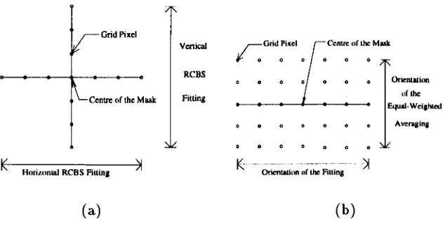
3.2 (a) The mask of the Chen/Yang edge detector, where the orientation of the fitting is determined by the Prewitt operator. (b) The mask of the proposed

roof edge detector. . . .. 21 3.3 From top to bottom: cubic B-spline and its first, second and third order

derivatives. 25

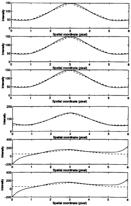
3.4 The fitted curve (solid line) on a roof edge (dashed line) using the RCBS fitting with various regularisation factors a. From top to bottom: a=10-7,

10-1

°,

10-13, 10-16, 10-19, and O. 28

3.6 The optimum edge maps produced when the test image (edge size=40) is contaminated with noise of various standard deviations (NSD's). (a) The test image. (b) The ideal edge map. (c) NSD=O. (d) NSD=5. (e) NSD=10.

(f) NSD=15. (g) NSD=20. 37

3.7 Top: The optimum regularisation factors obtained when the test image is contaminated with noise of various standard deviations (NSD's). Bottom: the corresponding FCR's when the optimum regularisation factors are used. In this test, the size of the roof edge and the threshold are 40 and 10

respectively. 37

3.8 Top: The optimum thresholds obtained in noise-free images with roof edges of various sizes. Bottom: The corresponding FCR's. In this test, the

regu-larisation factor 0 is 0.1. 38

3.9 The optimum edge maps obtained for noise-free roof edges of various sizes: (a) The ideal edge map; (b) Edge sizee IO; (c) Edge size=20; (d) Edge

size=30; (e) Edge size=40. 39

3.10 (a) The "Trevor" image. (b) The edge map of "Trevor" produced by the proposed roof edge detector (0=0.1; threshold-efi]. (c) The edge map of "Trevor" produced by the Haralick step edge detection scheme with the

threshold of 4. 40

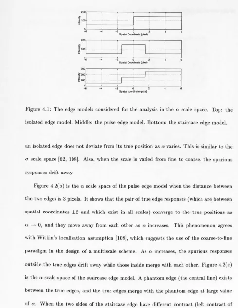
4.1 The edge models considered for the analysis in the 0 scale space. Top: the isolated edge model. Middle: the pulse edge model. Bottom: the staircase

4.2 The 0 scale space of: (a) the isolated edge model; (b) the pulse edge model;

( c) the staircase edge model; (d) the staircase edge model with a left contrast of 50 and a right contrast of 100. . . 49 4.3 Top of (a): the fitted curve of a pulse edge model with 0=0.001; Top of (b):

the fitted curve of a staircase edge model with 0=0.001; Bottom of (a),(b):

The second derivative of the fitted curve. 50

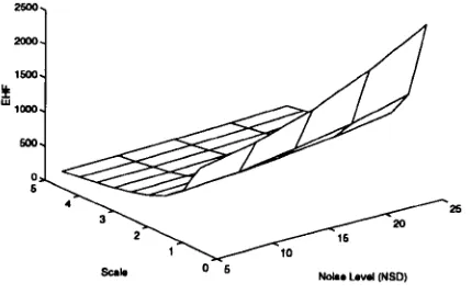
4.4 (a) The operator kernel of MRCBS employed in every scale. (b) The op-erator kernel of MRCBS which is employed only in the finest scale. The orientation of the fitting is along the orientation of the gradient. The equal-weighted averaging is used to achieve anisotropic diffusion .. 51 4.5 The schematic diagram of MRCBS. . . .. 52 4.6 The relationship between the noise level (NSD), the scale of a and the EHF

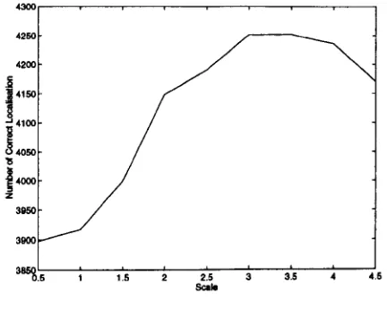
when the edge contrast is 100.. . . .. 54 4.7 The numbers of correct localisations when the RCBS fitting at various scales

is applied to 10000 different noisy edges. The contrast of the edge is 100 and the NSD is 10. . . .. 55 4.8 The relationship between a and NSD when TEHF is 308. . . .. 55 4.9 The ideal step edge and its fitted curves using the RCBS fitting with various

scales. Solid line: a step edge; dotted line: a = 1; dashdot line: 0 = 3;

dashed line: 0 =5 . 57

4.10 (a) The synthetic image used in the first test; (b) The ideal edge map. 63 4.11 (a) (b) and (c): The FCR's of the edge maps which are produced by the

Har-alick scheme, the Edge Focusing scheme and MRCBS in test 1 respectively.

4.12 The FCR's and ATR's ofthe edge maps which are produced by the Chen/Yang

edge detector in test 1 using various scales and thresholds. (a) Q = 1; (b)

Q = 2; (c) Q = 3; (d) Q = 4; (e) Q = 5; (f)-(j) are the corresponding ATR's

of (a)-(e) respectively. . . .. 65

4.13 The optimum FCR's and the corresponding ATR's of the edge maps

pro-duced by four different schemes in test 1 under various NSD's. MRCBS:

solid line; the Edge Focusing scheme: dashed line; the Chen/Yang edge

detector: dash dot line; the Haralick scheme: dotted line. . . 66

4.14 (a )-(d) The optimum edge maps of the first test produced by the Haralick

scheme (FCR=2.05, ATR=O.62), the Chen/Yang edge detector (FCR=O.15,

ATR=O.31), the Edge Focusing scheme (FCR=O.60, ATR=O.88) and

MR-CBS (FCR=O.05, ATR=O.43) respectively. These edge maps are obtained

when the NSD of the test image is 25. . . .. 67

4.15 (a) The test image 2 contaminated by Gaussian noise with NSD ranging

from 0 (on the left) to 25 (on the right); (b) The ideal edge map. . . .. 67

4.16 The FCR's and their corresponding ATR's of the edge maps produced by

four different schemes in test 2 using various thresholds. MRCBS: solid

line; the Edge Focusing scheme: dashed line; the Chen/Yang edge detector:

dashdot line; the Haralick scheme: dotted line. 68

4.17 (a)-(d) The edge maps of the second test produced by the Haralick scheme

(FCR=O.86, ATR=O.32), the Chen/Yang edge detector (FCR=O.14, ATR=O.13),

the Edge Focusing scheme (FCR=O.07, ATR=O.24) and MRCBS (FCR=O.02,

4.18 (a) The real image of "Trevor". (b), (c) and (d): The optimum edge maps produced by the Haralick scheme (threshold=5), the Chen/Yang edge de-tector (0=0.1, threshold e-t) and MRCBS (threshold=2) respectively. (e), (f) and (g) Three of the edge maps in the focusing process of the Edge Focusing scheme, where (G) is the final edge map. The threshold is 2 and the scales are a= 4.2, 1.4 and 0.7 respectively. (h) The final edge map (eT = 0.7) produced by the Edge Focusing scheme using a threshold of 1. (i) The edge map produced by MRCBS using a threshold of 5. . . .. 71

5.1 (a) An image with two textures- nuts and straw. (b) The boundary between the two textures. The variances of (a) using windows: (c) of size = 7 (pixels) and (d) size = 25 (pixels). (e) The edge map of (a) produced by the Laplacian of Gaussian scheme. (f) The luminance profile along the

central line of (a). . . .. 76

5.2 (a) A multiresolution representation of an image. The two textures are depicted as grey and white. The central regions of homogeneous textures are represented using large windows, whereas the border regions of textures are represented using small windows. (b) The feature space of (a), where large circle represent the texture feature of a large region in (a).. . . .. 82 5.3 The neighbouring blocks of a block in the (a) central area, (b) border area,

(c) corner area of an image. . . .. 84 5.4 Upper Left: The P(change) determined by the Metropolis probability

5.5 (a) LTV P(assign) at various levels. L=1: solid line; L=2: dashed line;

L=3: dashdot line. (b) LTV P(Jix) at various levels. L=3: solid line; L=6:

dashed line; L=10: dashdot line. 86

5.6 (a) An image with two textures- metal and straw. (b) The boundary

between the two textures. The segmentation map of (a) using a: (c)

ttuirqin.ratio of 0.17 (PCS=48); (d) marqin.ratio = 0.32 (PCS=96); (e)

marqin.ratio = 0.37 (PCS=97); and (f) marqiti.ratio = 0.45 (PCS=O). . . 92

5.7 The percentages of the correct segmentation (PCS's) of the segmentation

results of Figure 5.6( a) using various marqin.ratios. . . . .. 93

5.8 The intermediate segmentation maps of Figure 5.6(a) at different levels

using a marqin.ratio of 0.37. From (a)-(h): level 1-8. 95

5.9 The intermediate fixed regions (shown as grey) at different levels using a

marqin.ratio of 0.37. From (a )-(h): level 1-8. . . .. 96

5.10 (a) An image with textures of two different metals. The segmentation map

of (a) using a : (b) marqin.ratio of 0.17 (PCS=39)j (c) marqin.ratio

=

0.20 (PCS=59)j (d) marqin.ratio = 0.27 (PCS=69); (e) marqin.ratio

=

0.31 (PCS=93); and (f) marqinratio = 0.35 (PCS=93).. . . .. 98

5.11 The percentages of the correct segmentation (PCS's) of the segmentation

results of Figure 5.1O(a) using various marqin.s atios, 99

6.1 (a) Two OFC's (0.2u+0.25v-1 = 0 and 0.19u+0.26v-1 = 0) in the u-v

plane. (b) The OFC's with a slightly perturbed coefficients (0.2u

+

0.25v-1.03 = 0 and 0.19u

+

0.26v - 0.97 = 0). . 103

6.2 The parent-children relationship in a quad-tree: a unit for an over-determined

6.3 The u - v plane with a determined vector u-;,and a undetermined vector ul 106

6.4 A multiresolution representation of an image. The two motion fields are de-picted as grey and white. The central regions of homogeneous motion fields are represented using large windows, while the border regions of textures

are represented using small windows " 108

6.5 (a) An image frame in a sequence of synthetic images and (b) its previous

frame. . . .. 113 6.6 The segmentation map of the motion field tbasis.marqin =0.2pixel/frame

List of Tables

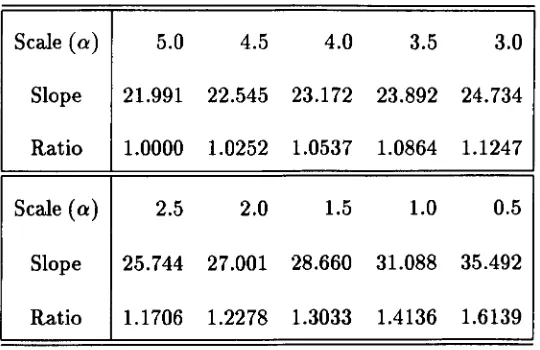
4.1 Slopes of the fitting at various scales, and the ratios of these slopes with

the slope at the coarsest scale.

4.2 Edge Focusing vs. MReBS ..

. 58

... 62

5.1 pes's of segmentation maps of Figure 6(a) using various marqin.ratios, . 93

5.2 pes's and the percentage of the fixed region at various levels. . . .. 94

5.3 pes's of segmentation maps of Figure 5.10(a) using various marqin.ratios, 99

6.1 The actual velocities, the estimated velocities, the error ratios and the

Acknowledgements

I would like to express my gratitude to my supervisor, Dr. T. Tjahjadi, for all his supports and ad vices throughout these three years. Without his patient proof reading and his comments, this thesis would not appear in such a well-written form. The financial support from the Linda Sumartini Foundation is gratefully acknowledged.

I would like to thank Dr. R.Staunton for his help while Dr. Tjahjadi was on sabbatical leave. I would also like to thank Chang- Tsun Li for all the stimulating discussions.

Declaration

This thesis is presented in accordance with the regulations for the degree of Doctor of Philosophy by the Higher Degree Committee at the University of Warwick. The thesis has been composed and written by myself based on the research undertaken by myself. The research materials have not been submitted in any previous application for a higher degree. All sources of information are specifically acknowledged in the content.

Summary

Chapter

1

Introduction

In recent years, digital images have been used extensively in medical, industrial and

telecommunication applications due to the rapid progress of digital techniques. Various im-age modality, including charge-coupled devices for light and thermal imaging, laser range imaging, Synthetic Aperture Radar imaging (SAR), as well as various medical imaging modalities such as the Magnetic Resonance imaging (MRI), the Computed Tomography (CT) and the Positron Emission Tomography (PET), have been developed to generate 2-D and 3-D images using signals with lower dimensions [18]. At the same time, various image processing techniques have been investigated to extract useful information from digital images, which normally contain some physical defects such as noise or blurring. The research discipline of image processing includes computed imaging, filtering,

which build up an artificial visual system. Tasks of computer vision include structure from motion, shape from shading, object tracking, etc. [40].

Although image processing groups and computer vision groups have slightly different emphases and attitudes toward research (the former tend to devise generic approaches, whereas the later are more interested in the interpretation of physical scenes from images), their close relationship cross fertilises each other. For example, segmentation and feature extraction are normally the starting points of both fields. In addition, the adaptivity in scale is generally the key component for an efficient computer vision or image processing algorithm.

Computer vision is an inverse process because the physical scene is reconstructed through images [6]. Since the physical information of a scene is incomplete in the im-age, assumptions have to be made during the reconstruction stage to estimate the missing information. An inverse problem is ill-posed in the presence of noise, violating the three requirements of well-posedness: (1) a solution exists, (2) the solution is unique, and (3) the solution depends continuously on the input data (see Section 3.2). Regularisation is a procedure for formulating a well-posed task by employing assumptions which guarantee a unique and stable solution to the task (see Section 3.2). Ithas been pointed out that reg-ularisation has a close relationship with the concept of scale [94]. This close relationship leads to the Bounded Diffusion theory presented in Chapter 4, which is one of the central issues addressed in this thesis.

tackled separately. In this thesis the tasks of edge detection and image segmentation using textures and motion fields are investigated. These tasks are low-level tasks, which determine the performance of the subsequent high-level tasks.

1.1

Edge Detection

Identifying and locating object boundaries in an image is an essential task in low-level computer vision because an object boundary provides an initial description of the scene. Object boundaries manifest themselves as significant discontinuities between image grey-levels of adjacent pixels, thus, the detection of these discontinuities (referred to as edges) attracts enormous attention from computer vision groups. A step edge corresponds to an abrupt change in grey-level (Le. a discontinuity), whereas a roof edge corresponds to the first order discontinuity in the image gradients. Marr uses edges to illustrate the concept of primal sketches [66], therefore the performance of the higher level computer vision relies on the accurate detection of edges. Physiological evidences also show that the recognition of edges plays an important role in mammalian vision. For example, Hubel and Wiesel have shown that mammalian cortex contains a population of feature detectors which is tuned to edges and bars of various width and orientation [66J.

tasks such as edge detection. This new concept is referred to as the Bounded Diffusion theory, where the adjustment of the regularisation effect according to the noise levels does not increase the size of the operator kernel.

1.2

Texture Segmentation

Image segmentation is the process by which an image is partitioned into disjoint regions, each of which has a homogeneous region property such as a texture or a motion field. It is an intermediate process toward a high-level interpretation of a scene. Although object boundaries manifest themselves as edges, edge detection alone cannot serve as a

complete image segmentation scheme. The reason being that edge detectors capture both boundaries and surface textures of an object. In addition, a procedure of edge linking is required after edge detection to compose a parametric contour (i.e. a chain of boundary locations) to complete the segmentation process (see Section 2.3). The difficulties of image segmentation is normally under-estimated because our natural aptitude to interpret a visual scene is excellent and spontaneous [105]. There are two approaches to tackle the problem of image segmentation: to consider region properties such as textures or colours; and to use information from multiple frames such as stereos or motion fields to recognise occlusion. In this thesis, texture segmentation and motion field segmentation are investigated.

This is a dilemma occurring in the joint space-frequency analysis, Le. the uncertainty principle (see Section 1.4), which indicates that a good texture segmentation can only be achieved using an adaptive multiscale (multiresolution) approach.

1.3

Motion Field Segmentation

The optical flow constraint equation (OFC) proposed by Horn and Schunck [43] is

com-monly used to derive the motion field from image sequences. OFC assumes that the image grey level of a moving point is stationary with respect to time, thus

dS(x,y,t) oS(x,y,t)dx oS(x,y,t)dy oS(x,y,t)

dt

=

ox dt

+

ay dt

+

at

=

0, (1.1)

where S(x, y, t) is the grey-level at an image pixel (x, y) at time t; and u

= ~~

and v

=

*

represent the two orthogonal components of the velocity of the image pixel.

each of which corresponds to a distinct motion field in the image. Thus, an adaptive multiresolution scheme is required to circumvent the uncertainty.

1.4

Uncertainty,

Scale and Multiresolution

As indicated in the previous three sections, researches on edge detection, texture seg-mentation and motion field segmentation all involve (by their nature or by a common misunderstanding among researchers) the uncertainty of the joint space-frequency anal-ysis. In this section, the uncertainty principle is examined in detail. Let h( x) denote the operator kernel (a real function with unit L2 norm) of the analysis, and H(w) be the Fourier Transform of h(x). Assume h(x) -+ 0 when x -+ ±oo. The spatial resolu-tion 6x and the feature resolution 6w in the time-frequency plane (also referred to as a spectrogram [84]) are defined as the variances of h(x) and H(w) respectively [20,98]:

6w2 [: w2IH(w)12dw

[: Ih'(xW dx.

Thus,

6x2 6w2 [: x2Ih(x)12 dx

x [:

Ih'(x)12 dx

>

If:

Xh(X)h'(X)dXI2 (Schwarz inequality) (1.2)

Since

equation (1.2) becomes

(1.3)

The above formula imposes a lower bound on the time-frequency product, which shows that high resolutions in both the spatial domain and the frequency domain cannot be achieved simultaneously in the joint space-frequency analysis. The equality of ( 1.3) is reached (Le. the uncertainty of the time-frequency product is minimised) when the two

functions involved in the Schwarz inequality of (1.2) are proportional to each other, Le. [20, 98]

h'(x)

xh(x) =constant,

where the solution of hex) is a Gaussian.

The issue of uncertainty, scale and resolution is the central issue of this thesis. It

has also been discussed in scale-space filtering methods (e.g. [59, 108]), wavelet meth-ods (e.g. [64, 84]), diffusion methods (e.g. [79, 102, 103]), as well as various multi-scalefmultiresolution techniques (e.g. [5, 62, 63, 110]). The underlying objectives of these theories are similar, which are the decomposition of an image into different spatial fre-quency channels (scales) so as to facilitate the joint space-frefre-quency or space-scale analysis. Generally, a scale is defined as the standard deviation of the Gaussian pre-filter a (e.g. [5,62]), a continuous parameter, which indicates the degree of smoothing of an image.

The standard deviation a of the Gaussian is proportional to the spatial resolution b.x.

In the literature, the spatial extent of the block-shaped window in the quad-tree image structure is also referred to as the resolution, which is a dyadic series. In this thesis the terminology of the scale is used in continuous situations, whereas the resolution is used to indicate the block size of the quad-tree.

noise level. Ifan image is noise-free, then the inner scale (Le. the smallest scale which is determined by the granularity of the image) always provides the most complete information of an image. Otherwise, an adequate scale is required to suppress noise. An accurate modelling of the noise level is thus essential for the indication of the scale. This will be discussed in Section 4.3.1.

1.5

Organisation of the Thesis

This thesis tackles three computer vision tasks of edge detection, texture segmentation and motion field segmentation. In this thesis, uncertainty, scale and adaptivity are the central concepts which are closely linked together. Due to the local nature of edges (see Section 1.1), Bounded Diffusion is proposed to provide a local scale factor for edge detection, where the spatial extent of the operator kernel is independent of the scale. Texture seg-mentation and motion field segmentation are susceptible to uncertainty, thus an adaptive multiresolution clustering method is devised to circumvent the uncertainty.

Chapter

2

Edge Detection

2.1

Finite Difference Edge Detector

A digital image is a two-dimensional (2-D) array of grey levels, which correspond to the sampled light intensities in light images, or the depth values in range images. Normally the grey levels are indicated by a third coordinate which is perpendicular to the 2-D image plane. Therefore, the digital image g(Xi' Yi) is viewed as the sampled data from a 3-D continuous surface f(x, y), where x and yare spatial coordinates, and Xi and Yi are the grid points of x and y.

As defined in Section 1.1, a step edge corresponds to an abrupt change in grey level, whereas a roof edge corresponds to the discontinuities in image gradients. The abrupt change occurs in grey-level g(Xi' Yi) when the underlying surface f(x, y) is very steep. A step edge is thus defined as the set of pixels (x, y) where the gradient of f(x, y) exceeds a certain threshold value:

of (x, y) Bf(x, y) h h Id

ox

+

By

~ t

res 0 •

difference method, Le.

(2.1)

Alternatively, they can be determined by convolving a weighting mask (also known as a window or an operator kernel) with the image. These masks are square matrices, e.g.

-1 -k -1

a/(x, y)

ax ~ g(Xj, yd

*

0 0 0

1 k 1

-1 0 1

a/(x,y)

ay ~ g(Xj, Yi)

*

-k 0 k

-1 0 1

where

*

denotes convolution; k is a positive constant. Compared with the finite difference method of equation (2.1), these weighting masks introduce a smoothing effect along the orientation which is perpendicular to the derivative so as to suppress noise. Different value of k have been proposed heuristically. For example, k

=

2 in the Sobel operator and k

=

1 in the Prewitt operator [30J. Masks with different sizes are also proposed for different degrees of smoothing. However, these approaches are incapable of calibrating the size of the masks according to the noise level so as to avoid excessive bluring.

2.2

Laplacian of Gaussian Operator

pixels correspond to the zero values of the second order derivative along the gradient in the underlying surface

I,

i.e.

where nis the coordinate along the gradient [94]. Normally the above process is simplified to detecting the zero-crossings of the Laplacian of the image, i.e. \j2

I,

as an edge.

The detection of an edge using the Laplacian operator or the finite difference operator is an ill-posed task because the inherent differentiation enhances the high-frequency compo-nents of the image including noise. The results are thus highly noise-sensitive. A rigorous definition of well-posedness is presented in Section 3.2. The method of regularisation con-verts an ill-posed task into well-posed. Torre and Poggio showed that regularisation can be achieved by convolving the data with a cubic-spline filter, which has a shape similar to a Gaussian [94].

Marr and Hildreth [66] proposed the Laplacian of Gaussian operator (LoG), an isotropic operator, for edge detection. The idea is to convolve an image with a Gaussian smoothing pre-filter G( a, x, y) for the regularisation, and then calculate the Laplacian of the smoothed image to produce an edge-enhanced image EE(Xi' Yi) (a band-passed image), i.e.

where a is the standard deviation of the Gaussian. The LoG operator \j2G(a, X, y) is

which is also known as the "Mexican hat" operator due to its shape [66]. Note that the 2-D Gaussian can be decomposed to two I-D Gaussians, i.e.

1 _($2+112) 1 _,..2 1

.;;:5-G(a,x'Y)=-2 2e 2(12 = rn-- e2ci1"x rn-- e2(1 =G(a,x,O)xG(a,O,y).

Similarly

{)2 {)2

({)X2

+

{)y2) [G(a,x,O) X G(a,O,y))

{)2 {)2

£) 2G(a,x,O)xG(a,O,y)+G(a,x,O)x ll2G(a,O,y).

ux uy

This shows that the 2-D convolution of an image with \j2G(a, x, y) can be simplified as four 1-D convolutions. The LoG operator can also be approximated by the Difference of Gaussian (DoG) kernel [66], which is the basic principle of the Laplacian pyramid [13].

Figure 2.1 shows the image of "Trevor" and the edge-enhanced image obtained from the convolution of "Trevor" with the LoG kernel. In Marr and Hildreth's approach, the edge map is further derived using the set of pixels with zero values in the edge-enhanced

image.

(a) (b)

Figure 2.1: (a) The image of "Trevor"; (b) The edge-enhanced image produced by the

LoG filter.

a large amount of blurring by increasing the value of (1, which however causes the edges to

be displaced from its original positions (see Chapter 4). Marr and Hildreth have discussed the edge behaviour under various value of (1 [66]. This concept is further developed by

Witkin as the scale-space theory [108].

2.2.1 Uncertainty and Gaussian

Canny employed the numerical optimisation method to design an optimised 1-D kernel for an edge detector [16]. Three criteria, i.e, the suppression of noise, the localisation of edges, and one single response to an edge, are chosen for the optimisation. The result showed that the optimised kernels for step and roof edges are approximated by the first and the second order derivatives of a Gaussian respectively. Canny's first two criteria correspond to the uncertainty which occurs in edge detection, Le. a large degree of smoothing is required to suppress noise, whereas a small degree of smoothing is preferable for locating the edges accurately. Thus Canny's numerical result confirms the theoretical prediction of the uncertainty principle that the Gaussian is the optimum kernel (see Section 1.4).

Canny also suggested the use of the ~G( (1,n) operator instead of the LoG operator

for edge detection, where n is the coordinate along the gradient. This agrees with the natural definition of an edge, i.e.

f,&.,

which is also accepted by Torre and Poggio [94], Haralick (see Section 2.3), and the MRCBS proposed in Chapter 4.

2.3

Surface Fitting Edge Detector

Reconstructing the physical scene from digital images is the objective of computer vision. Under this premise, an intuitive procedure is to fit the sampled grey levels with a continu-ous surface. Haralick proposed the facet-model based edge detector [39], which comprises two steps. First, a set of 2-D Chebychev orthogonal polynomials are employed to fit a window of image pixels g. The reconstructed underlying surface j, referred to as a facet, is a linear combination of these Chebychev polynomials, where a series of coefficients c determine the weights of the polynomial. These coefficients are determined by the least-square fitting, which minimises a well-posed quadratic energy function E =

II

Ac - 9

11

2,

where

II . II

denotes the 12-norm, and matrix A maps the coefficients from c space to g

space. Hence, the minimum of E occurs when c = (AT A)-l AT 9 [90], which indicates that c is continuously dependent on g. The least-square fitting provides a smoothing effect similar to the result of the Gaussian pre-filtering.

Second, the gradient of the facet j and the second derivative along the gradient ori-entation (Le.

fnt)

are determined. If a zero-crossing occurs on ~ at a pixel, and the gradient of the pixel is larger than a threshold, then this pixel is classified as an edge pixel. Figure 2.2(b) shows the edge map produced by the Haralick edge detector.

(a) (b)

Figure 2.2: (a) The image of "Trevor"; (b) The edge map produced by the Haralick edge detector (the threshold is 4).

1. A I-D plane is used to least-square-fit a window of image pixels;

2. Determine the gradient orientation of the fitted plane;

3. A third-order I-D polynomial is used to least-square-fit the same pixels to refine the estimation of the gradient;

4. A I-D tanh function is used to least-square-fit the same window;

5. A quadratic polynomial is used to least-square-fit the image pixels along the orien-tation determined at step 3;

6. Compare the error of the least-square-fitting in steps 4 and 5. Ifthe error in 4 is greater than in 5, then an edgel is determined. The I-D tanh function is thus used to determine the orientation and the magnitude of the edgel.

2.4

Active Contour Model

The active contour scheme is devised to extract a contour directly from the image grey levels [50]. This scheme minimises the functional E:

where the contour is represented parametrically by

v(s)

=

(x(s),y(s)),

with arc length parameter s E [0,1]. Eintern is the internal energy due to the elastic deformation and the bending of the contour. Eimage corresponds to the target feature such as a step edge or a roof edge. The external constant term Econllt is defined as the distance between the contour and a given spatial position. This is to facilitate the man-machine interaction. The solution

v(s)

is determined by minimising E. For example, the energy functional of a roof-edge contour is:

E =

j(a(s)lvs(sW

+

,8(s)l

v

ss(sW)ds

+

Lg(v(s))

If

where a(s) and (3(s) are weightings; v,,(s) and v"s(s) are, respectively, the first and the second order derivatives of the contours

v(

8).

g( v(

8)) denotes the grey level along

v(

8).

are inserted automatically. Thus, a contour with a complex shape is gradually extracted as the scale decreases.

2.5

Discussion

This chapter reviews the advantages and drawbacks of the finite difference operators, the Laplacian of Gaussian operator, the Haralick's facet model, the tanh l-D surface fitting approach, as well as the active contour model for edge detection. The use of the finite difference operators for edge detection is intuitive but ill-posed, thus it fails on noisy images. The Laplacian of Gaussian operator, which combines the Gaussian pre-filter and the Laplacian differentiator, is well-posed. However, the isotropic Laplacian of \/2 is an approximation of the true edge differentiator of ~ [94]. The Haralick operator comprises the facet model (for a local surface fitting) and the ~ differentiator. Nalwa and Binford proposed a complex approach which is based on the l-D tanh surface fitting. The local surface around an edge is fitted and therefore, the parameters of the edgels are available for the subsequent edge linking process. The active contour scheme, which is based on the minimisation of a regularisation functional, produces a contour directly from the grey level image according to the required features (e.g. step or roof edges). However, a few snaxels have to be specified to serve as the initial condition.

Chapter

3

Roof Edge Detection and

Regularisation

3.1

Roof Edge Detection

A roof edge is an important feature in various applications. For example, it is argued that human facial expressions in images are better depicted by roof edges than by step edges [78]. The extraction of roof edges from digital terrain models plays an important role in lithology, structural geology and geo-morphology [83]. Roof edges are also important in the analysis of aero-magnetic images [44] and the segmentation of range images [41, 77].

A roof edge is generally defined as a discontinuity in the first order derivative of a I-D grey-level profile

f

[77, 54]. This definition is adopted in this thesis. However, in certain instances a sign change in the first order derivatives on the two sides of the discontinuity is also required [38], i.e. f'(to+) Xf'(to-) ::;0, where the discontinuity occurs at the position

the principle orientation (the principle orientation is defined in Section 3.4.1).

6

Spatial coordinate (pixel)

Coordinate on Principal orientation

Figure 3.1: An example of a roof edge.

Various schemes for detecting roof edges (or ridges and valleys) have been proposed. Pearson and Robinson proposed a valley detector, which uses a set of criteria to examine the relative grey levels of a group of neighbouring pixels [78]. These criteria determine the local extremum of the second order derivative of the underlying grey-level profile, which indicates the occurrence of a roof edge. Unfortunately, this scheme requires three thresh-olds to be given heuristically. Furthermore, it is an ill-posed task due to the embedded differentiation process (see Section 3.2).

Recently, Chen and Yang proposed a step edge detector based on the Regularised Cubic B-Spline (RCBS) fitting [17]. However, this scheme has two limitations which degrade its performance. First, the Prewitt edge detector, an ill-posed operator, is used to indicate the local gradient, along which the subsequent fitting is applied. The accuracy of this scheme is thus limited. Second, the grey-levels along the gradient, which are required for the fitting, do not coincide with the grid pixels of the image (Figure 3.2(a». Interpolation is thus required, which increases the computation time. This chapter presents a roof edge detector, derived from Chen and Yang's step edge detector, which overcomes the above two limitations. The proposed roof edge detector employs the 1-D RCBS fitting on the horizontal and the vertical orientations of a window of image pixels to generate two I-D signals (see Figure 3.2(b», which provides sufficient information of the 2- D facet to enable edge detection.

Grid Pixel

Vertical

o

Orientation

of the Equal-Weighted

RCBS r-GridPixel

v-

0 0

Centre of theMask

Centre of the Mask Filling

o Averaging

o 0 0 0

Orientation of the Filting

K

Horizontal RCBS Filling

(a) (b)

Figure 3.2: (a) The mask of the Chen/Yang edge detector, where the orientation of the fitting is determined by the Prewitt operator. (b) The mask of the proposed roof edge

3.2

Well-posedness and Regularisation

Hadamard defined a well-posed task to have the properties of existence, uniqueness and continuity [6J, where

existence: for each datum 9 in a given class of functions G, there exists a solution x in

a prescribed class X;

uniqueness: the solution x is unique in X;

continuity: when the error on the data 9 tends to zero, the induced error on the solution

x also tends to zero.

As indicated in Chapter 1, the tasks of computer vision are inverse processes in the sense that the 3-D physical scene is reconstructed from digital images. The information contained in an image is insufficient to produce a unique and stable solution which repre-sents the physical scene, unless an adequate physical knowledge is used to constrain the solution space. The incorporation of constraints is referred to as the regularisation process. For example, due to the process of differentiation in edge detection, a small perturbation of 9 (e.g. noise) induces an unpredictable change of the edge location x. Thus, it is an ill-posed process which violates the criterion of continuity. From the point of signal pro-cessing, the process of differentiation corresponds to a high-pass filtering, which enhances the noisy components of the signal. Hence, the task is ill-posed and the solution of x is numerically unstable.

from the data g(.) such that f(-) ~ g(.). Tikhonov's format includes an additional term which comprises a suitable norm

II . II

as well as a stabilising function

Q,

Le.

E

=11

f(·) - g(.)

112 +a

II

Qf(·) 112, (3.1)

where a determines the degree of regularisation and E is the energy. Thus f(·) is deter-mined such that E is minimised.

L2 norm is generally chosen as

II . II

and d2 / dx2 as

Q

for the sake of simplicity [94], Le.

(1- D)

(2 - D)

In this way, the space of the solution for a regularised functional is constrained by sup-pressing the second order derivative of f(·), Le. a smoothness constraint. The physical justification is that the noise-free image is band-limited by the optics, therefore, all its derivatives of the underlying surface should exist and be bounded [94].

Toore and Poggio argued that the determination off(·) via the Tikhonov regularisation is equivalent to convolving the digitised image g(.) with a a cubic spline filter, which is very similar in shape to a Gaussian filter [94]. On the other hand, the role of Gaussian smoothing can be replaced by a regularised fitting. This is the basic concept of Bounded Diffusion, which will be discussed in Chapter 4.

3.3

Regularised Cubic B-Spline Fitting

The Regularised Cubic B-Spline (RCBS) fitting, which employs the principle of the regu-larisation theory [6,92], is used to reconstruct the grey-level profile f(x) from a discrete array of data g(Xj) in a well-posed way, i.e.

E =~)f(xj) - g(Xj))2

+

aJ(dYx~X))2dX,

J

where a is a positive number and Xj are the sampled pixels of a spatial coordinate x. The variational approach is commonly used to solve the functionals [92]. However, tech-niques such as curve fitting can transform a functional problem into the minimisation of a quadratic energy equation, where the solution is easily determined by linear algebra. Among various curves available for the fitting, a spline under a certain premise has a least value of the second order derivative according to the Holladay theorem [1]:

Holladay Theorem

Let 6. : a

=

Xl

<

X2

< ... <

XM

=

b, and a set of real numbers {g(xk)}(k =

1,2, ... ,M) be given. Then among all the functions f(x) with a continuous second

deriva-tive on [a.b], and such that f(xk) =9(Xk), the spline function S6(X) with junction points

at Xk and with S'b,(a)

=

S'b,(b)

=

0 minimise the intergal

Here the spline function S6(x) is defined to be composed of cubic polynomials in each

sub-interval Xk-l ~ X ~ Xk (k

=

2,3, ... ,M), and satisfies S~(Xk+)

=

S~(Xk-) as well

as S'b,(Xk+)

=

S'b,(Xk-), (k :2,3, .... ,M-I).

Since the sampling rate of a digital image is fixed, the interval [Xk-l, Xk]is equidistant. Hence a spline S6(Xk) is a linear combination of a third-order basis function provided that the derivatives of the basis function are zero at the boundary points. This concept motivates the RCBS fitting [17, 56], which uses the cubic B-spline

n

(Figure 3.3) as the

basic elements of the fitting:

o

2 ~ Ixi

n

=

-lxI

3/6

+

IxI

2 -

21xI

+

4/3 1

<

[z]

<

2

!o·:f

_:

_:

₁

i 0

-2 -1.5 -1 -0.5 0 0.5 1.5 2

Spatial coordinate (pixel)

t

~I

_:

_:

_I

i_I

-2 -1.5 -1 -0.5 0 0.5 1.5 2

Spatial coordinate (pixel)

t

~L_F__ ~:

___.___~==;:_,_____::::::.,....::=.._::;;2~~ ___._:

____J:1

i-

2--2 -1.5 -1 -0.5 0 0.5 1 1.5 2

Spatial coordinate (pixel)

1

:1:---_5L--!- _

___,,::==~==~~:---,----:-,:-_j

-2 -1.5 -1 -0.5 0 0.5 1.5 2

SpaUal coordinate (pixel)

Figure 3.3: From top to bottom: cubic B-spline and its first, second and third order

derivatives.

By shifting the basis function over the interval [I,M],

ej(x) =Q(x - i) iE Z.

The solution f( x) in equation (3.2) is then represented as the linear combination of the basis functions:

M+l

f(x) =

L

cjej(x),

j=O

(3.3)

where c, is the coefficient of the basis function ej.

In this way, the regularised functional in equation (3.2) becomes a quadratic energy equation:

M M+l M M+l d2.( .)

" " 2 "( " e, xJ 2

E = L) L..J Cjej(Xj) - g(Xj))

+

a L...J

!-

Cj dx2 ),

J=l

,=0

J=l 1=0

(3.4)

as the second order derivatives at the positions of xj, and a is used to adjust the relative

importance between the two terms. Given g(Xj) and a, Ci is then determined. The solution f( x) and its derivatives can then be easily obtained by multiplying e, with the corresponding derivatives of ei:

M+l

f(n)(x)

=

I:

cie~n)(X),

;=0

where f(n)(x) and e~n)(x) represent the nth order derivatives of f(x) and ei(x), respectively.

3.3.1

Quadratic Energy Equation

Define

c=

A=

g(xt)

G=

where A, A2 and G are known, and C is the unknown variable. In this way, equation (3.4) can be represented as

Since the row vectors of [A A2] are independent of each other, the matrix P is positive definite as long as a

>

O. Therefore,

This is a standard quadratic energy equation and the graph is a paraboloid in the (M+2) dimensional hyperspace. The minimum of E occurs at C =p-1AG [90].

3.3.2

Ill-Conditioness

A quadratic energy equation is well-posed. However, it can be ill-conditioned, which means that a small perturbation in the input signals results in a large variation of the output. When a -+ 0, P -+ AAT, which is a singular matrix because the rank of A is M,

and the dimension of the matrix AA T is M+2 by M+2 such that det{AA T) = O. The singularity of AAT causes the computation of C, which requires the inverse of P, to be ill-conditioned. Since there is no clear boundary between ill-conditions and well-conditions [6], the MATLAB software is used to simulate the fitting with a decreasing value ofa. The results (Figure 3.4) show that when aequals to 10-7,10-1°,10-13, satisfactory fittings are achieved. However, when a is further decreased to 10-16,10-19as well as 0, the results of the fitting are unsatisfactory, i.e. the results do not represent roof edges. Similarly, a -+ 00 causes the computation to be ill-conditioned. Values of a in the range 10-7 to 20

showed similar results to Figure 3.4{ a).

r~k2S

1

0123458

=c:===-:

f~==:

'---~--j

=~-.-+: ...

I_~=,:

---:--j

0123458

[image:46.521.160.375.148.487.2]

SpalIII coordinal1 (pIxeO

Figure 3.4: The fitted curve (solid line) on a roof edge (dashed line) using the RCBS fitting with various regularisation factors a. From top to bottom: a=1O-7, 10-1

°,

10-13, 10-16,

method which changes equation ( 3.3) to:

M

f(x)

=

LCiei(X)

i=1

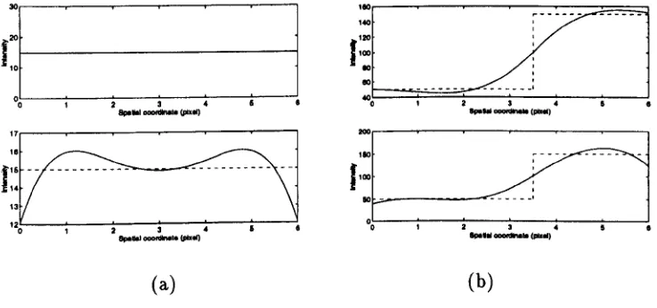
Therefore, only M cubic B-splines are used instead of M+2 as in equation (3). However,

the use of EM will not result in an optimum fit, because the RCBS fitting is regularised

and therefore, is well-posed. The solution of a well-posed problem is guaranteed to exist, is

unique, and is continuously dependent on the input data (see Section 3.2). Ifthe boundary

cubic B-splines (i.e. eo(x) and eM+1(x)) is removed from the fitting procedure as suggested

in [17], then the accuracy of the fitted curve degrades as illustrated in Figure 3.5. In this

thesis the RCBS fitting with M+2 cubic B-splines is used.

'1 : : : : :

0123" 5'

I

I~~l

0

nnnZJ

1 2 3 " I •

...-(pIX",

..."'-(-,

[image:47.521.79.448.305.478.2]

(a) (b)

Figure 3.5: Top of (a): the fitted curve (solid line) of a straight line (dashed line) using

the RCBS fitting; Top of (b): the fitted curve (solid line) of a step edge (dashed line) using

the RCBS fitting; Bottom of (a) and (b): the fitted curve obtained by the exact mapping

(EM) method. Here a=O.1.

3.3.3 Theorem of Linear Fitting

The regularised fitting is a linear process in the sense that the fitted curve is proportional

Theorem 1 Linear Fitting Theorem

Consider the regularised fitting

the solution f of the functional E(f,g) is linearly dependent on the image grey-level g. Proof:

Given go.

Let fo be the candidate solution of 90 which minimises E, i.e. E(Jo,90) is minimised. then

for 9m =a X go

+

b, ( a, b E R)

there exists fm

=

a X fo

+

b, such that

is also minimised.

3.4

The Design of a Roof Edge Detector

• f" ~

threshold;

• zero-crossing occurs in

I"'.

Since an image is a 2-D signal, the above 1-D criteria cannot be used directly. There are two approaches to solve this problem: (1) augment the 1-D criteria to 2-D; and (2) use a 1-D signal in an appropriate orientation to represent the 2-D image. The latter approach is used in this design to simplify the computation.

3.4.1 Principal Cross Section

The grey level of a 2-D image describes a 3-D surface. To use a 1-D signal

I

(a grey-level profile) to represent this 3-D surface for roof edge detection, a cross-sectional plane is required on which

f

is the projection of the 3-D surface. This cross-sectional plane, referred to as the principal cross section, is perpendicular both to the 2- D image and the isophote curves (i.e. the curves which connect pixels of the same grey level). The orientation of the principal cross section is thus referred to as the principal orientation (see Figure 3.1).

Let S(x, y) be the 3-D grey-level surface, where x and yare spatial coordinates. Let

x

be the principal orientation, and

iJ

be the orientation of the isophote curve, then ~~ =

f#

= O. Given an arbitrary direction t inclined at an angle () to the direction of

x,

then

x

= tcos() and

iJ

= tsinB.

Therefore,

dS

dt

as

as.

ax

x

cos()

+

ay

x

smB

as

and

(3.6)

Denote

,

as

Jp

=

ox'

JP"

=

02SOX2'

and

, dS

J()

=

Tt,

J()t" _- ddt2S2•

Therefore, equations (3.5) and (3.6) become

f~(x, Y)

=

fp(x, y) X cosO,

J~'(x, y)

=

fp(x, y) X cos20. _(3.7)

These relationships infer that

f

along the principal orientation (fJ = 0) has the maximum first and second order derivatives. Note that these relationships are obtained under the assumption that the isophote curves are parallel to the roof edges. Although this is not always true, the assumption generally approximates the real cases.

3.4.2 Horizontal-Vertical Decomposition

Therefore,

Uo(x, y»2

+

UO+90o(X, y»2 U;'(X, y»2COS2()

+

U;'(X, y»2sin2()

=

U;'(x, y»2, (3.8)

fo'(x, y)

+

fO~90o(x, y) = fp(x, y)cos2()

+

fp(x, y)sin2() = fp(x, y). (3.9)

Equation (3.8) and (3.9) show that f;'(x,y) and fp(x,y) can be obtained from the derivatives along any two perpendicular orientations. Note the two formulae in equation (3.8) and ( 3.9) are identical to the definition of the gradient and the Laplacian respectively, where I;'(x, y) corresponds to the gradient, and Ip(x, y) corresponds to the Laplacian. To simplify the computation, the two perpendicular orientations are chosen to be the horizontal and the vertical orientations so that the grey levels on the sampled image can be directly used for the regularised fitting.

3.4.3

The Algorithm

In the proposed roof edge detector, the RCBS fitting is applied along the horizontal and the vertical orientations to reconstruct two continuous grey-level profiles (Figure 3.2(b

».

The derivatives of the fitted curve

f

along these two orientations are then obtained as described in Section 3.3. Since the basis function, the cubic B-spline, is a third order piecewise polynomial, the third order derivative of the fitted curve

f

is not continuous at

the grid pixels (see Figure 3.3).

The criteria for detecting a roof edge (Section 3.4) are then applied along the principal orientation. The first criterion requires

lp,

determined using equation (3.9), to be greater than a threshold. The second criterion requires a zero-crossing in /"', i.e. fP'(to+) X

examined along the horizontal and the vertical orientations. Ifa sign change occurs along either of the two orientations, the second criterion is satisfied. The first criterion is then used to detect the roof edge.

The magnitude of ftp is used as an indication of roof edges in the proposed scheme, where ftp is determined from two regularised 1-D signals, and equals approximately to the Laplacian of Gaussian \j2G(U,X, y)

*

S. The difference between ftp and \j2G(U,X, y)

*

S is the shape of the kernel, Le. a cross kernel (Figure 3.2(b)) is used to compute

f'f"

while

a square kernel is used to compute \j2G(u, X, y)

*

S.

The pseudo codes of the proposed roof edge detector are:

begin

Input (Image(x, y), a, threshold);

Assign n = the size (in pixels) of the image;

For (x

=

1,2, ....n)(y

=

1,2, ....n) do begin

Apply the RCBS fitting along the horizontal orientation;

Determine fhorizonta/(x, y), fh~rizonta/(x-, y), and fh~rizonta/(x+, y); Apply RCBS fitting along the vertical orientation;

Determine f~~rtica/(x, y), f~~rtica/(x, y-), and f::rtica/(x, y+);

IfU;:;rizonta/(x-, y) X f;:;rizontal(x+, y)

<

0)

or U~~rtical(x, y-) X f::rtical(x, y+)

<

0)

then

begin

f'f,(x, y)

=

If;:orizontal(x, y)

+

f~/ertica/(x, y)1

Ifftp(x, y)

>

threshold

else Set EdgeMap(x, y)=Not an Edge;

end

end

Output (EdgeMap( x, y));

end

3.5

Performance Evaluations

The values of the regularisation factor Cl! and the threshold are required for the proposed

roof edge detector. The value of Cl! determines the degree of smoothing, therefore, a large

value of Cl! should be used when the image is noisy. Conversely, if the image is noise-free,

a small value of Cl! should be used so as to preserve the image details. The value of the

threshold reflects the size of an edge, which is defined as the difference of the slopes at the two sides of the roof edge [54J. The larger the edges to be detected, the larger the threshold.

falsely-detected pixels to the number of correctly-detected pixels, i.e.

Fe R

=

number of falsely-detected pixels number of correctly-detected pixels

ntrn-l-nfp

ntp-l-nta-l-nne

The lower the value of FeR, the better is the performance of the operator. Ifthe value of FeR is greater than 1, the operator is considered to have failed, because the number of falsely-detected pixels exceeds the number of correctly-detected pixels. Here the param-eters which generate an edge map with the least value of FeR are considered optimum parameters.

In test 1, a synthetic image which contains a roof edge with a slope of 20 at both sides of the edge, i.e. the size of the edge is 40, is used to represent a typical roof edge (Figure 3.6(a)). The image is contaminated with zero-mean Gaussian noise of various standard deviation (NSD), and the FeR's of the edge maps produced by the proposed roof edge detector are determined. In the noise-free case, the edge map has a FeR of

o

(i.e. the edge map is perfect in the context of FeR) when the regularisation factor is

0.1 and the threshold is 10. The threshold is then set to 10 for all the noise levels since the regularisation factor alone should reflect the noise level. The optimum regularisation factors and their corresponding FeR's are then measured under various NSD's. The results (Figure 3.7) show that the optimum regularisation factor increases as the NSD increases. The corresponding optimum edge maps are shown in Figure 3.6.

00

(a) (b) (c) (d)

.~~.'"...:':'~':_'':.:

's : ..

~. .}

.~': .~

"<.:..) ....,./

.

:..

..~.

.'>:...'

>~v.:

',Ii- ,.

...

, ... :3'

(e)

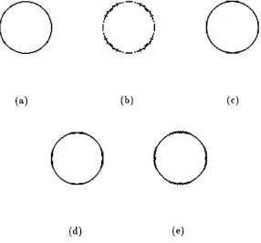
(f) (g)

Figure 3.6: The optimum edge maps produced when the test image (edge size=40) is contaminated with noise of various standard deviations (NSD's). (a) The test image. (b) The ideal edge map. (c) NSD=O. (d) NSD=5. (e) NSD=10.

(f)

NSD=15. (g) NSD=20.

5

~4 • • • • • • • I • •

LL.

~3

tU

j2

"

II

2 4 6 8 10 12

Noise Standard Deviation

2

1.5

a:

o 1 LL.

0.5

00

2 4 6 8 10 12 14 16 18 20

Noise Standard Deviation

Figure 3.7: Top: The optimum regularisation factors obtained when the test image is con-taminated with noise of various standard deviations (NSD's). Bottom: the corresponding

points become more and more similar, and hence more and more difficult to distinguish. Figure 3.9 shows the corresponding optimum edge maps.

6r---.---~----~----~~----~--__.

5.5

15 20 25 30

Size of the Roof Edge

35 40

0.1

15 20 25 30

Size of the Roof Edge

35 40

~o

Figure 3.8: Top: The optimum thresholds obtained in noise-free images with roof edges of various sizes. Bottom: The corresponding FeR's. In this test, the regularisation factor

et is 0.1.

In test 3, a real image of "Trevor" (Figure 3.10(a» is used as a test image, and the corresponding roof edge map generated by the proposed scheme is shown in Figure 3.10(b). Figure 3.10( c) shows the step edge map produced by the Haralick step edge detector [39] for comparison. It shows that the features on the step edge map and the roof edge maps are different. For example, the step edge map shows the wrinkles on the shirt, while the roof edge map shows the stripes on the shirt. The pattern on the tie appears to be better

o

o

(a) (b) (c)

00

[image:57.510.126.412.208.474.2]

(d) (e)

Figure 3.9: The optimum edge maps obtained for noise-free roof edges of various sizes:

(a) The ideal edge map; (b) Edge size=10; (c) Edge size=20; (d) Edge size=30; (e) Edge

(b) (c)

3.6

Summary

In this chapter, the concept of regularisation is examined. This concept relates to both the numerical stability (Le. the well-posedness of the task) and the scale (Section 3.2). Section 3.3.1 shows the use of Cubic B-spline fitting transforms a functional of regularisation into a quadratic energy function. A roof edge detector is devised which does not rely on the Prewitt edge detector as in the Chen/Yang step edge detector [17]. The roof edge detector

Chapter

4

Bounded Diffusion

4.1

Multiscale Edge Detection

The multiscale aspect of edge detection was first examined by Rosenfeld and Thurston [85]. They analysed the edge responses using the box-shaped kernels with various sizes, and observed that some edge points are not detected when a large kernel (i.e. low spa-tial resolution) is applied. Marr and Hildreth proposed the Laplacian of Gaussian edge detector, in which a Gaussian pre-filter is applied to regularise the ill-posed task of edge detection and to suppress noise (see Section 2.2). They observed that when an image is convolved with a Gaussian kernel of various standard deviation (1, different edge maps,

defined as the zero-crossings of the Laplacian, are produced. A small (1 results in an edge

map with more details than one which is obtained using a large (1, but there are also more

noise-induced responses [66]. Marr and Hildreth suggested that the zero-crossings which exist over several scales should be considered as physically significant [66]. These edges are referred to as salient edges.

a scale coordinate, where the scale is the standard deviation a of the Gaussian pre-filter. In a scale space, the zero-crossings of the second order derivative of a signal produce traces which reflect the relationship between the scale and the step edges. Witkin pointed out the "well-behavedness" of the a scale space, Le. when the scale is varied from coarse to fine, new local extrema are created while existing ones remain [108]. Babaud et al. [3]

proved that for a I-D signal, this property only holds when the signal is convolved with a I-D Gaussian. Yuille and Poggio [109] further confirmed that this property also holds when an image is convolved with a 2-D Gaussian, and proved that it can be applied to all

level-crossing contours. Koenderink [53] proved that the Gaussian is the Green's function of the diffusion equation, i.e. in the 1-D case

where a represents the scale, x is the spatial coordinate and 1/1 is the signal. Hence, the theory of scale space motivates the study on the diffusive aspects of an image.

Based on the evolutionary behaviour in the scale space, a few multiscale edge detection schemes have been proposed. The essence of these schemes is to locate edges as accurately as possible while suppressing noise. Bergholm proposed the Edge Focusing scheme [5] which first obtains an edge map from a coarse scale, and then consecutively decreases the scale to recover the true positions of edges. Lu and Jain [63] proposed the scheme for "reasoning about edges in scale space" (RESS), which involves a large amount of decision

making to classify edges according to their behaviour in the scale space.

kernel size is large. However, an edge is a local feature. A large kernel includes irrelevant information into the edge detection and therefore, the detected locations of edges deviate from their true positions. This is why in both Bergholm's, and Lu and Jain's approaches, extra computations are required to recover the true positions of edges. The Q scale space

is proposed in Section 4.2 to cope with this problem. In the Q scale space, the size of

the operator kernel is independent of the value of Q, which corresponds to the degree of

smoothing.

The value of a scale corresponds to the noise level of the image [16]. The higher the noise level, the stronger the smoothing effect should be. Hence, the noise level determines the lower bound of the scale, beyond which the estimated locations of edges are no longer accurate because the noise is not sufficiently suppressed. The Edge Focusing scheme employs a series of scale (0' = 4.2, 3.85, 3.5,3.2,2.8,2.5,2.1, 1.75, 1.4,1.0,0.7) which is heuristically chosen

[5].

Therefore, if an image is very noisy, the edge locations recovered in the finest scale are not accurate. This is referred to as an "over-focused" phenomenon in

[5]. In some images, the noise level varies from one region to another, thus the scale needs to be adjusted adaptively. This adaptivity is referred to as the "variable blurring" in

[5].

To prevent over-focusing and to enable variable blurring in edge detection, a multiscale edge detector is proposed in Section 4.3 where the finest scale is adaptively adjusted according to the local noise level.

to suppress noise. Note that the criterion of an edge being the zero-crossings of the second order derivative is susceptible to noise, thus it is normally accompanied by the criterion of a large gradient (see Sections 2.2 and 2.3). To prevent noise clusters in edge detection, a series of thresholds should be used in every scale in a multiscale scheme.

A multiscale edge detector with a fixed-size kernel is proposed to address the above three issues. The scale is adjusted adaptively according to the local noise level. A series of thresholds are used in every scale, which controls the amount of details to be preserved in

the edge map. The proposed multi scale edge detector is still based upon the Regularised Cubic B-Spline (RCBS) fitting described in Section 3.3, where a set of cubic B-splines (Figure 3.3) is used to approximate the underlying I-D grey-level profile. A regularisation term, controlled by a factor o, is introduced to suppress the effect of noise:

(4.1)

where g( xj) denotes the grey level at the spatial coordinate xj. The fitted curve f( x) is determined by minimising the functional E. The proposed edge detector is thus referred to as the Multiscale edge detector based on Regularised Cubic B-Spline fitting (MRCBS).

In equation (4.1), Cl! reflects the degree of smoothing, which is determined by the value

of (J' in Gaussian pre-filtering methods. Also, both the Gaussian pre-filtering and the

regularised fitting convert the ill-posed nature of edge detection to well-posed [94]. As the kernel size is independent of o , the image is diffused within a small range, Le. a bounded diffusion. Therefore Cl! could be interpreted as a scale, where the terminology of scale is

4.2

Bounded Diffusion in a Scale Space

4.2.1 Uncertainty and Bounded Diffusion

A signal contains both global and local information, where a scale such as (7 normally

reflects the spatial extent of the operator kernel. The essence of a multiscale analysis is to interpret a signal using the operator kernel with varous spatial extents. As indicated in equation (1.3), the spatial resolution of 6.x and the frequency resolution of

6w

in a joint space-frequency (space-scale) analysis are constrained by the uncertainty principle [20]. This can be illustrated by two simple examples. The Fourier transform (FT) of a Dirac function (b( x)) is 1 for all frequency w. Similarily, the FT of a function that approximates an edge:

edge(x)

= {

1 when x> 0, -1 when x

<

0; is 2/jw, where j is the unit imaginary number.