COMPARISON OF POWER VALUES IN GENERALIZED LINEAR MIXED MODEL (GLMM) UNDER THE
DIFFERENT ESTIMATION METHODS
1
Md. Abu Manju* and
1Assistant Director, Statistics Department, Bangladesh Bank, Head Office, Dhaka, Bangladesh,
2Professor, Department of Statistics, University of Chittagong, Bangladesh
ARTICLE INFO ABSTRACT
In longitudinal studies, the Generalized Estimating Equation (GEE) and Maximum Likelihood (ML) methods are commonly used to estimate the parameters of Generalized Linear Mixed Models (GLMM). Power and sample size estimat
longitudinal study design and planning of modern clinical trials. In this paper, the power of the Wald Test for two different estimation methods of parameters in GLMM was compared. The data employed in this study
was found in which the power values were better under ML approach than GEE approach for the GLMM.
INTRODUCTION
Generalized linear mixed-effects models, more commonly known as generalized linear mixed models (GLMM), are widely commonly frequently used in longitudinal data analysis. The GLMM are natural combinations of two modeling strands, the linear mixed models and the generalized linear models. Linear mixed models (e.g., Hartville, [5]; Laird and Ware, [8] are linear regression models that include normally distributed random effects in addition to fixed effects. A natural application is to longitudinal data where random effects vary between subjects and induce within subject dependence among repeated measurements after conditioning on observed covariates. Generalized linear models Nelder and Wedderburn, [11]; Wedderburn, R. W. M. [20] unify regression models for different response types such as linear models for continuous responses, logistic models for binary responses, and log-linear models for counts.
are the generalized linear models that include multivariate normal random effects in the linear predict
contributions explicitly discussing this idea are Wong and Mason [19] and West [22] in frequentist and Bayesian settings, respectively. The term “generalized linear mixed model” appears to have been coined by Gilmour, Anderson, and Rae [21], although it’s widespread use is probably due to the highly cited paper by Breslow and Clayton [2]. In social statistics and other areas, generalized linear mixed models are also known as hierarchical, multilevel, or random
models.
*Corresponding author: [email protected] [email protected]
ISSN: 0975-833X
International Journal of Current Research
Vol. 3, Issue,
Article History: Received 15th
September, 2011 Received in revised form 30th
October, 2011 Accepted 27th
November, 2011 Published online 31th December, 2011 Key words:
Generalized Linear Mixed Model, Generalized Estimating Equation, Power Function,
Noncentral Chisquare Distribution.
RESEARCH ARTICLE
COMPARISON OF POWER VALUES IN GENERALIZED LINEAR MIXED MODEL (GLMM) UNDER THE
DIFFERENT ESTIMATION METHODS
d. Abu Manju* and
2Soma Chowdhury Biswas
Director, Statistics Department, Bangladesh Bank, Head Office, Dhaka, Bangladesh, Professor, Department of Statistics, University of Chittagong, Bangladesh
ABSTRACT
In longitudinal studies, the Generalized Estimating Equation (GEE) and Maximum Likelihood (ML) methods are commonly used to estimate the parameters of Generalized Linear Mixed Models (GLMM). Power and sample size estimation constitutes an important component for longitudinal study design and planning of modern clinical trials. In this paper, the power of the Wald Test for two different estimation methods of parameters in GLMM was compared. The data employed in this study were diabetes mellitus data with three consecutive follow ups. A pattern was found in which the power values were better under ML approach than GEE approach for the GLMM.
Copy Right, IJCR, 2011, Academic Journals
effects models, more commonly known as generalized linear mixed models (GLMM), are widely commonly frequently used in longitudinal data analysis. The GLMM are natural combinations of two d the generalized linear models. Linear mixed models (e.g., Hartville, [5]; Laird and Ware, [8] are linear regression models that include normally distributed random effects in addition to fixed effects. A natural application is to longitudinal data where the random effects vary between subjects and induce within-subject dependence among repeated measurements after conditioning on observed covariates. Generalized linear Wedderburn, R. W. M. r different response types such as linear models for continuous responses, logistic models for linear models for counts. GLMMs are the generalized linear models that include multivariate normal random effects in the linear predictor. Early contributions explicitly discussing this idea are Wong and Mason [19] and West [22] in frequentist and Bayesian settings, respectively. The term “generalized linear mixed model” appears to have been coined by Gilmour, Anderson, ough it’s widespread use is probably due to the highly cited paper by Breslow and Clayton [2]. In social statistics and other areas, generalized linear mixed models are also known as hierarchical, multilevel, or random-coefficient
The simplest cases of GLMMs are the random
models with a single normally distributed random effect. Random-intercept models are sometimes referred to as variance components, error components, or random models. Early applications of such m
random-intercept probit models discussed by Lawley [9], in psychometrics. Similar models were later considered by Heckman and Willis [27] in econometrics. Pierce and Sands [13] and Anderson and Aitkin [1] discussed random
logit models, and Hinde [6] and Brillinger and Preisler [28] discussed random-intercept Poisson models.
Introducing random effects with conjugate distributions into special cases of generalized linear models has a very long history, including the negative binom
Greenwood and Yule, [4] and the beta
proportions Skellam, [18]. Although these models, which are strictly not GLMMs, a major limitation is that they cannot be extended to random-coefficient models where the effects o covariates vary randomly between subjects.
Albert [23] discussed a generalized estimating equation (GEE) approach to fit the GLMM and both classes of models (Subject-Specific & Population Average) for discrete and continuous outcomes. The
subject-assumed to follow a Gaussian distribution, simple relationships between the Population Averaged (PA) and Subject Specific (SS) parameters are available. Actually the SS model is the simplest example of GLMM. Sometimes we have to make a definite decision one way or another about a particular hypothesis in the GLMM; in this situation a test of hypothesis is appropriate. Although in science we never accept ternational Journal of Current Research
Vol. 3, Issue, 12, pp.182-188, December, 2011
INTERNATIONAL
OF CURRENT RESEARCH
COMPARISON OF POWER VALUES IN GENERALIZED LINEAR MIXED MODEL (GLMM) UNDER THE
Director, Statistics Department, Bangladesh Bank, Head Office, Dhaka, Bangladesh, Professor, Department of Statistics, University of Chittagong, Bangladesh
In longitudinal studies, the Generalized Estimating Equation (GEE) and Maximum Likelihood (ML) methods are commonly used to estimate the parameters of Generalized Linear Mixed ion constitutes an important component for longitudinal study design and planning of modern clinical trials. In this paper, the power of the Wald Test for two different estimation methods of parameters in GLMM was compared. The data were diabetes mellitus data with three consecutive follow ups. A pattern was found in which the power values were better under ML approach than GEE approach for the
Copy Right, IJCR, 2011, Academic Journals. All rights reserved.
The simplest cases of GLMMs are the random-intercept models with a single normally distributed random effect. intercept models are sometimes referred to as variance components, error components, or random-effects models. Early applications of such models include the intercept probit models discussed by Lawley [9], in psychometrics. Similar models were later considered by Heckman and Willis [27] in econometrics. Pierce and Sands [13] and Anderson and Aitkin [1] discussed random-intercept models, and Hinde [6] and Brillinger and Preisler [28]
intercept Poisson models.
Introducing random effects with conjugate distributions into special cases of generalized linear models has a very long history, including the negative binomial model for counts Greenwood and Yule, [4] and the beta-binomial model for proportions Skellam, [18]. Although these models, which are strictly not GLMMs, a major limitation is that they cannot be coefficient models where the effects of covariates vary randomly between subjects. Zeger, Liang, and a generalized estimating equation (GEE) approach to fit the GLMM and both classes of models Specific & Population Average) for discrete and -specific parameters are assumed to follow a Gaussian distribution, simple relationships between the Population Averaged (PA) and Subject Specific (SS) parameters are available. Actually the SS model is the simplest example of GLMM. Sometimes we have to make a definite decision one way or another about a particular hypothesis in the GLMM; in this situation a test of hypothesis is appropriate. Although in science we never accept INTERNATIONAL JOURNAL
a hypothesis outright, but rather continually modify our ideas and laws as new knowledge is obtained, in some situations, such as in clinical practice, we cannot afford this luxury. To understand the concepts of validity and power, it will be helpful if we consider the case in which a decision must be made, one way or the other, with the result that some wrong decisions will inevitably be made. Clearly, we wish to act in such a way that the probability of making a wrong decision is minimized. Repeated measurements arising from longitudinal studies occur frequently in applied research. Methods to calculate power in the context of repeated measures are available for experimental settings where the covariate of interest is a discrete treatment indicator. However, no closed form expression exists to calculate power for generalized linear models with non-zero within-cluster correlation that are common in epidemiological and observational studies in which the covariate of interest varies over time and is often measured on a continuous scale, and where the researchers control for several potential confounders. Gastan, McLaren &
Delfinob [29] discussed a procedure to calculate power of the test for the normal linear mixed model, and the logistic regression model, both with repeated measurements and non-zero within-cluster correlation. Correlated binary data are common in biomedical studies. Such data can be analyzed using Liang and Zeger’s generalized estimating equations (GEE) approach. An attractive point of the GEE approach is that one can use a misspecified working correlation matrix, such as the working independence model (i.e., the identity matrix), and draw (asymptotically) valid statistical inference by using the so-called robust or sandwich variance estimator. Wei Pan [24] derived some explicit formulas for sample size and power calculations under various common situations. Gwowen Shieh [15] described A direct extension of the approach described in Self, Mauritsen, and Ohara [17] for power and sample size calculations in generalized linear models is presented. The major feature of the proposed approach is that the modification accommodates both a finite and an infinite number of covariate configurations. Gwowen Shieh [30] wrote another paper in which A method is proposed for improving sample size calculations for logistic and Poisson regression models by incorporating the limiting value of the maximum likelihood estimates of nuisance parameters under the composite null hypothesis. The method modifies existing approaches of Whitteinore [25] & Signorini [31] provides explicit formulae for determining the sample size needed to test hypotheses about a single parameter at a specified significance level and power. Özdemir and Eyduran [12] described a study comparatively analyzed in point of power of test of Chi-Square and Likelihood Ratio Chi-Square statistics. Steven G. Self & Robert H. Mauritsen [16] proposed an approach for estimating power/sample size within the framework of generalized linear models. This approach is based on an asymptotic approximation to the power of the score test under contiguous alternatives and is applicable to tests of composite null hypotheses. The power properties of traditional repeated measures and hierarchical linear models have not been clearly determined in the balanced design for longitudinal studies. Hua Fang, Gordon P. Brooks & Maria L. Rizzo [7] proposed a procedure A Monte Carlo power analysis of traditional repeated measures and hierarchical multivariate linear models under three variance-covariance structures. In methodology we have discussed the estimation procedure of GLMM by ML & GEE approaches and the procedure of
conducting the power function for Wald Chisquare test. Actually we have tried to show whether there exist any differences in power values of the same test due to different methods of estimation. In results section we have illustrated our methodology for subject-specific logistic regression model.
METHODOLOGY
Let
y
it denote the tth observation in the ith cluster,i
T
t
1
,
,
. Letx
it denote a column vector of values of explanatory variables, for fixed effect model parameters
.Let
u
i denote the vector of random effect values for cluster i.This is common to all observations in the cluster. Let
z
itdenote a column vector of their explanatory variables. Often, the random effect is univariate. Conditional on
u
i , a GLMM resembles an ordinary GLM. Letu
it
E
(
Y
itu
i)
. The linear predictor for a GLMM has the form
it
x
itz
itu
ig
(1.0)for link function
g
. The random effect vectoru
iis assumed to have a multivariate normal distributionN
(
0
,
)
. The covariance matrix
depends on unknown variance components and possibly also correlation parameters. Denote),
(
)
var(
Y
itu
i
v
it where the variance functionv
(
)
describes how the (conditional) variance depends on the mean and
is an unknown dispersion parameter. The variabilityamong
u
i induces a nonnegative association among the responses, for the marginal distribution averaged over the subjects. This is caused by the shared random effectu
i for each observation in a cluster. In (1.0), the random effect enters the model on the same scale as the predictor terms. This is convenient but also natural for many applications. For instance, random effects sometimes represent heterogeneity caused by omitting certain explanatory variables.Estimation of GLMM by MLE
Maximum Likelihood Method: Model fitting is rather complex for GLMMs. The main difficulty is that the likelihood function does not have a closed form. Numerical methods for approximating it can be computationally intensive for models with multivariate random effects. In this section we outline the basic ideas of ML fitting of GLMMs. The GLMM is a two-stage model. At the first two-stage, conditional on the random effects, observations are assumed to follow a GLM. That is, observation
y
it in cluster i has distribution in the exponential family with expected valueu
it linked to a linear predictor,
itx
itz
itu
ig
assumed independent from a
N
(
0
,
)
distribution. For example the simplest example of the GLMM is the Subject-Specific logistic regression model or logistic regression model with the random intercept and the form of the model)
1
.
1
...(
)]
1
(
[
log
it
P
Y
it
u
i
x
it
u
iwhere
u
i~
iid
N
(
0
,
2)
For a discrete variable, denote the vector of all the observations by y and the vector of all the random effects by u. Let
f
(
y
u
;
)
denote the conditional mass function of y, given u. Letf
(
u
;
)
denote the normal density function for u. The likelihood functionl
(
,
;
y
)
for a GLMM is the probability mass functionf
(
y
;
,
)
of y, viewed as a function of
and
. This mass function refers to the marginal distribution of y after integrating out the random effects,
y f y f yu f u du
l(, ; ) ( ;, ) ( ;) ( ; ) … (1.2) It is often called a marginal likelihood. For example, the
likelihood functions
l
(
,
2;
y
)
for the logistic-normal model (1.1)
i yt it i
i it it u x u x * ) exp( 1 ) exp( ( ) ) ; ( ) exp( 1
1 1 2
i i y i it du u f u x it
The likelihood function is evaluated numerically and maximized as a function of
and
. Many methods have been developed to do this. We next discuss one of the popular methods.Gauss–Hermite Quadrature Method
The integral determining the likelihood function has dimension that depends on the random effects structure. Gauss Hermite quadrature is a method for approximating the integral of a function
f
(
)
multiplied by another function having the shape of a normal density. The approximation is a finite weighted sum that evaluates the function at certain points. In the univariate normal random effects case, the approximation has the form
q k k kf
s
c
du
u
u
f
12
)
(
)
exp(
)
(
with weights
c
k and quadrature points
s
k that are tabulated. The approximation improves as q, the number of quadrature points, increases. The approximated likelihood can be maximized with standard algorithms such as NewtonRaphson, yielding ML estimates
ˆ
and
ˆ
. Inverting an approximation for the observed information matrix provides standard errors for the ML estimates. For complex models, second partial derivatives for the Hessian may be computednumerically rather than analytically. Adequate approximation
usually requires larger q for standard errors than for
ˆ
.Estimation of GLMM by GEE
GEE Approach: Zeger, Liang and Albert (1988) discussed a procedure to estimate GLMM by Generalized estimating Equation (GEE) approach. To use the GEE approach for the GLMM, we calculate the marginal moments,
i andV
i, from the conditional moments and the random effects distribution, F. We then solve the equation)
3
.
1
...(
...
0
)
)(
(
)
(
1 1 * *
K i i i ii
V
Y
U
discussed by Liang and Zeger (1986). Given the conditional moments in
it
x
itz
itu
ig
and a distribution, F, for the random effects, the marginal expectation,
i has the form ofit
=
y
it =
y
it|
u
i
=
h
1x
it
z
itu
idF
(
u
i)
The marginal covariance matrix is
(
|
)
cov(
|
)
cov
i i i ii
Y
u
Y
u
V
with s, t element
)
(
)
(
)
(
)
(
)
)(
(
, i it i is is it it t s iu
dF
u
g
t
s
I
u
dF
u
u
V
where
u
it
h
1(
x
it
z
itu
i)
and I(s=t) is the indicator function with value 1 if s = t and 0 otherwise. Having evaluated
iandV
i for each subject/cluster, we solve the GEE given in (1.3) for
. Note that the GEE is a function of F, which is assumed to be known at a given iteration. For example If we consider the Subject-Specific logistic regression model/Logistic normal regression model andassuming
u
i~
iid
N
(
0
,
2)
, the expression for the marginal mean simplifies by Zeger et al. (1988) and given by
)
exp(
1
)
exp(
)
(
it it itit
E
Y
c
x
c
x
where
21 2
6
.
0
1
c
Expanding the link function in a Taylor series about
u
i
0
gives the approximation
i it i it i it i it iu
x
u
h
x
h
g
u
x
u
h
x
h
Y
)
(
)
(
)
(
)
(
cov
)
cov(
1 1 1 1
i i i i ii
Z
Z
L
A
V
L
ˆ
Where
Li= diag
i itt
n
x
u
u
u
h
,...,
1
,
,
)
(
1
Using
V
~
i, as an approximation toV
i, we have that conditional on F,K
(
ˆ
)
is asymptotically multivariate Gaussianwith mean 0(if an exact expression for
it is used and smallbias otherwise) and with variance that can be consistently estimated by 1 1 1 1 1 1 1 1 1 ˆ
ˆ
ˆ~
ˆ
*
ˆ
ˆ~
)
ˆ
)(
ˆ
(
ˆ~
ˆ
*
ˆ
ˆ~
ˆ
ˆ
K i i i i K i i i i i i i i i K i i i iV
V
Y
Y
V
V
V
The approximate estimates of variance covariance matrix of the random effects is
ˆ
Z
i
Z
i
1Z
i
L
i
V
i
A
i
L
i1Z
i
Z
i
Z
i
1and the estimates of the scale parameter is
K i n t it it it i it it ig
z
D
z
L
y
1 1 2 2ˆ
ˆ
ˆ
ˆ
ˆ
Hypothesis Tests After estimating the vector of regression coefficients
ˆ
, it may be of interest totest hypotheses concerning the elements of
. Considerhypotheses of the form
H
0:
C
d
where
C
is ac
p
matrix of constants imposingc
linearly independent constraints on the elements of
andd
is a1
p
vector of constants. There exists a established property that the ML estimates are approximately normally distributed with respective mean and variance and Liang and Zeger (1988) shown that the GEE estimates also normally distributedwith respective mean and variance. Again since
ˆ
is asymptotically normal, so the Wald test statistic
C
d
C
Var
C
C
d
Q
C
ˆ
ˆ
ˆ
1
has an asymptotic
c2 distribution ifH
0 is true.Power of the Wald Test
Now we are interested to test the null hypothesis
d
C
H
0:
against alternative hypothesisd
b
C
H
1:
, whereC
is ac
p
matrix of constants imposingc
linearly independent constraints on the elements of
andd
is ap
1
vector of constants. To construct the power function of the Wald test, at first we have to know thedistribution of Wald test under alternative hypothesis
H
1. PHILLIPS, P. C. B. [14]discussed the exact distribution of the Wald test under alternative hypothesis. According to PHILLIPS, P. C. B. [14], the probability density function of the Wald statistic (w) underH
1 is given by
kj k f q
f k f
q jk C I
N w N w m m w pdf q q , ( ) 2 1 2 / 1 ! ! / 2 / 1 1 2 / exp 2 2
det 12 j,k , , det N/2
f L X I L L X IL mm I X C L I X L
X0
)
(
2 2
q
with the non centrality parameter is
b
C
C
b
b
V
b
m
m
1 12
)
(
where
L
V
12C
12V
12C
12According to Shieh, G. [15], to calculate the power function, at first we have to find the
100
(
1
)
th percentile of acentral chi-square distribution with p d.f., denoted by
2
1 ,
c
and then find the non centrality parameter
2 of the non central chi-square distribution with cd.f such that the100
th percentile, denoted by 2
(
2)
,
c is equal to
2
1 ,
c ,
mathematically it can be written as
,
1
(
1)
) ( 2
2
2
F
p
c
where
p
1 denotes the
1
th
percentile of the centralchi-square
2 1 ,
c and
F
c2(2)(
p
1)
is the cumulativedensity of the noncentral chisquare distribution with c degrees
of freedom and noncentrality parameter
2 atp
1.RESULTS AND DISCUSSION
Table 1. Fixed Effect Estimates of Subject-Specific Logistic Regression Model Obtained by Maximum Likelihood (ML) Methods with Associated Wald Test
Variables Estimated Coefficients
Standard Error (Coefficients /S.E)^2
Odds- Ratio P-value
Intercept (Fixed)
-0.129146 0.171574 0.567009 --- 0.45162
[image:5.612.216.402.197.238.2]Age -0.001502 0.003171 0.224676 0.998499 0.63560 Sex -0.248922 0.076806 10.504081 0.779640 0.00119*
Table 2. Random Effect Estimates of Subject-Specific Logistic Regression Model Obtained by Maximum Likelihood (ML) Methods
Variables Estimated Variance
Std. Dev.
Intercept (Random)
[image:5.612.139.476.285.330.2]0.018059 0.13438
Table 3. Variance Covariance Matrix of the Estimated Fixed Effect Parameters of Subject-Specific Logistic Regression Model Obtained by Maximum Likelihood (ML) Methods
Constant Age Sex
[image:5.612.127.492.372.436.2]Constant 0.0294376090 -0.0004494745 -0.0022280906 Age -0.0004494745 1.005209e-05 -0.0000244092 Sex -0.0022280906 -0.0000244092 0.0058992143
Table 4. Fixed Effect Estimates of Subject-Specific Logistic Regression Model Obtained by Generalized Estimating Equation (GEE) Approach with Associated Wald Test
Variables Estimated Coefficients
Standard Error
(Coefficients /S.E)^2
Odds- Ratio P-value
Intercept (Fixed)
-0.146814 0.197544 0.552341 --- 0.457362
Age -0.001503 0.004138 0.131994 0.998497 0.716373 Sex -0.247109 0.094552 6.830247 0.781055 0.008962
Table 5. Random Effect Estimates of Subject-Specific Logistic Regression Model Obtained by Generalized Estimating Equation (GEE) Approach
Variables Estimated Variance
Std. Dev.
Intercept (Random)
0.015135 0.12302
Table 6. Variance Covariance Matrix of the Estimated Fixed Effect Parameters of Subject-Specific Logistic Regression Model Obtained by Generalized Estimating Equation (GEE) Approach
Constant Age Sex
Constant 0.039152492 -0.000766086 -0.002768442 Age -0.000766086 1.709722e-05 -4.592932e-05 Sex -0.002768442 -4.592932e-05 8.966033e-03
Table 7. Comparison of Power for Testing the Null Hypothesis
0:
2
0
Against the Alternative Hypothesis
1:
2
0
by the Wald Chisquare Test When the Parameters are Estimated by Maximum Likelihood (ML) & Generalized Estimating Equation (GEE) Approaches Respectively
[image:5.612.217.402.480.523.2] [image:5.612.139.478.567.612.2] [image:5.612.69.523.668.713.2]
The variable sex is dichotomous, where 0 stands for female and 1 stands for male.
The logistic regression model is given by
i i SS i SS SS SS i i
i i
i age sex it age sex
Y
it( 1| , ,)log ( )0 1 2
log
such that the population-averaged odds ratio for sex given by
SS ii i i i i
i i i i i i SS sex
age sex Y P age sex Y P
age sex Y P age sex Y P
OR exp 2
) , , 0 | 0 ( ) , , 0 | 1 (
) , , 1 | 0 ( ) , , 1 | 1 (
represents the ratio of the odds of a given patient having with confirmed diabetic if the patient is a male compared to the odds of the same confirmed diabetic if the patient is a female. Alternatively, ratio of the odds among male patients with confirmed diabetic having the same value of unobserved random effect to the ratio of the odds of those confirmed diabetic patients with the same value of unobserved random
effect who are female. Let
ˆ
2 be the estimated coefficient of the covariate sex under ML or GEE approach. We are interested to test the null hypothesis
0:
2
0
against the alternative hypothesis
1:
2
0
by the Wald test.We have discussed the issue of power calculations in GLMM with correlated data. We have presented relevant formulas for several important special cases. In this paper, we have developed a systematic approach to power analysis for the most popular longitudinal data approaches, the GEE and MLE. By extending existing methods to accommodate more practical considerations, this unified approach improves the limitations of these methods and provides a quite general approach for power and sample size estimation in GLMM for repeated measures. The approach presented here allowed us to compute power for a relatively complex study for which no exact methods are available. This study compares the performance of different methods of estimation for GLMM using the power values.
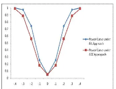
According to the diabetes data considered in the study, we may conclude that if we are interested to calculate power values of the Wald test, we should use the ML method of estimation because the Wald test gives greater power values under this method of estimation than the method GEE. Under both the method of estimations the fixed effect covariate sex shows the significance contribution to the diabetes status by the Wald Chisquare test and gives the approximate estimates -0.25.
Table 7 shows that power differences increases if the parameter values tend to the magnitude 0.25 which means that the proposed Wald Chisquare test detects highly the effect size under the ML methods of estimation. Most longitudinal studies, consider varying follow up times for the subjects which produces the missing data. In the article, the GEE and ML methodologies with non missing data was addressed. Hence, a common, constant number of follow ups for each subject was considered.
Power Curves Comparison for Testing the Null Hypothesis
0
:
2 0
Against the Alternative Hypothesis0
:
21
by the Wald Chisquare Test When the Parameters are Estimated by Maximum Likelihood (ML) and Generalized Estimating Equation (GEE) Approaches RespectivelyREFERENCES
1. Anderson DA, Aitkin M. Variance components models with binary response interviewer variability. J.R. Statistical Soc (1985); Series B, 47, 203-210.
2. Breslow N, Clayton G. Approximate inference in generalized linear mixed models. J. Amer. Statist. Assoc (1983); 88: 9-25.
3. Chamberlain G. Analysis of covariance with qualitative data. Re®. Econ. Stud (1980); 47; 225-238.
4. Greenwood M, Yule GU. An inquiry into the nature of frequency distributions representative of multiple happenings with particular reference to the occurrence of multiple attacks of disease or of repeated accidents. J. Roy. Statist. Soc (1920). Ser A 83; 255-279.
5. Hartville DA. Maximum likelihood approaches to variance component estimation and to related problems. Journal of American Statistical Association (1977). 72; 320-388.
6. Hinde J. Compound Poisson regression models. Pp. 109-121 in GLIM 82: Proc. International Conference on Generalised Linear Models (1982), ed. R. Gilchrist. New York: Springer-Verlag.
7. Fang H, Brooks GP, Rizzo, ML. A Monte Carlo power analysis of traditional repeated measures and hierarchical multivariate linear models in longitudinal data analysis, Journal of Modern Applied Statistical Methods (2008), Vol. 7, No. 1; 101-119.
8. Laird NM, Ware FH. Random effects models for longitudinal data. Biometrics (1982).38; 963-974. 9. Lawley DN. A general method for approximating the
distribution of likelihood ratio criteria. Biometrika (1956). 43; 295-303.
10. Liang KY, Zeger SL. Longitudinal data analysis using generalized linear models. Biometrika (1986). 73; 13-22. 11. Nelder JA, Weddervurn RWM. Generalized linear models. J. R. Statistical Soc (1972). Series A, 135, part 3, 370-384.
[image:6.612.340.528.45.190.2]Sciences Research 1(2): 242-244, 2005, © 2005, INSInet Publication
13. Pierce DA, Sands BR. Extra-Bernoulli variation in regression of binary data. Technical Report 46, Statistics Deptartment (1975), Oregon State University, Cornwallis, OR.
14. Phillips PCB. The exact distribution of the Wald statistic. Econometrica (1986). Vol. 54, No. 4, 881-895. 15. Shieh G. On power and sample Size calculations for
likelihood ratio tests in generalized linear models. Biometrics (2000). 56, 1192-1196.
16. Self SG, Mauritsen RH. Power/sample size calculations for generalized linear models, Biometrics (1988). 44, 79-86
17. Self SG, Mauritsen RH, Ohara J. Power calculations for likelihood ratio tests in generalized linear models. Biornetrics (1992). 48, 31-39.
18. Skellam JG. A probability distribution derived from the binomial distribution by regarding the probability of success as variable between the sets of trials. J. Roy. Statist. Soc (1948). Ser. B 10: 257-261.
19. Wong GY, Mason WM. The hierarchical logistic regression model for multilevel analysis. J. Amer. Statist. Assoc (1985). 80: 513-524.
20. Wedderburn RWM. Quasi-likelihood functions, generalized linear models, and the gauss-newton method. Biometrika (1974). 61: 439-447.
21. Gilmour AR, Anderson RD, Rae AL. The analysis of binomial data by a generalized linear mixed model. Biometrika (1985). 72, 3, 596-599.
22. West L. A review of J. Kiefer's work on conditional
frequentist statistics. INDIANA 47907-1399. PHILADELPHIA, PENNSYLVANIA (1985). 19104-6302.
23. Zeger SP, Liang KY, Albert PS. Models for longitudinal data: A generalized estimating equation Approach. Biometrics (1988). 44, 1049-1060.
24. Pan W. Sample size and power calculations with correlated binary data, Controlled Clinical Trials 22:211–227, Elsevier Science Inc (2001).
25. Whittemore AS. Sample size for logistic regression with small response probability. Journal of the American Statistical Association (1981).76, 27-32.
26. Zeger SL. The analysis of discrete longitudinal data: commentary. Statistics in Medicine (1988). 7, 161-168. 27. Heckman JJ, Willis RJ. "Estimation of a Stochastic Model of Reproduction An Econometnc Approach, 99-146 National Bureau of Economic Research (1976), Inc
28. Brillinger DR, Preisler HK. Maximum likelihood
estimation in a latent variable problem. Studies in Econometrics, Time Series and Multivariate Statistics (1983). Academic Press: New York; 31–65.
29. Gastañaga VM, McLaren CE, Delfino RJ. Power calculations for generalized linear models in observational longitudinal studies. 27-33 (2006)
30. Shieh G. A simple approach to power and sample size calculations in logistic regression and Cox regression models. Statistics in Medicine (2004) Volume: 23, Issue: 11, Pages: 1781-1792
31. Signorini. Sample size for Poisson regression, Biometrika (1991). 78, 446-50