HIGH NONLINEAR INCREMENTAL CONTROL OF A SOLAR THERMAL POWER PLANT USING SOFT COMPUTING FUZZY TUNING TECHNIQUES
Rodney Stirrup and Andrew J. Chipperfield
Computational Engineering & Design Research Group, School of Engineering Sciences, University of Southampton, Highfield, Southampton, SO17 1BJ, United Kingdom Telephone: + 44 (0) 23 8059 8301, Fax: +44 (0)23 8059 7082, e-mail: [email protected]
Abstract – Society is experiencing massive growth of global industrialised populations, which is putting increasing pressure on western governments to pursue more persuasive means to maintain and increase their share of the world’s diminishing fossil fuel reserves. To combat this, there is a growing body of enlightened researchers who are directing their abilities towards the development of alternative and preferably renewable energy types of supply systems. Many of these real world systems exhibit varying degrees of non-linearity. An example of this is the significant variations in the dynamic characteristics of a distributed collector field within a solar thermal power plant. Here a Sugeno-type fuzzy incremental controller was tuned using an ANFIS (Adaptive Neural Fuzzy Inference System) to optimise the fuzzy controller’s pre-clustered input membership functions, while a multiobjective genetic algorithm with an enhanced decision support system was used to fine tune the parameters of its first order output membership functions. The resulting solution choice produced an incremental fuzzy controller which was used to successfully control the plant exclusively in its high nonlinear regions, i.e., where the oil flow fell below 5 litres per second. This allowed the plant to function in environments where local solar radiation conditions have always been regarded as marginal. A feedforward term was also used to control plant disturbances caused by solar irradiation, mirror reflectivity etc.
1. INTRODUCTION
Previous research from Norway has demonstrated that a gain scheduling approach, (Johansen, et al., 2000), can be used to successfully control a solar power generation plant (Camacho, Berenguel and Rubio, 1997), over a large part of its operating range. However, the results of this type of control deteriorate somewhat when the plant is operated in its more nonlinear regimes. It is therefore proposed in this work to concentrate on designing a controller which is better suited to such slow system dynamics, i.e., when the plant is operating in regions of high nonlinearities. Earlier work on controllers that fit these requirements include: the fuzzy PD, (Malki and Chen, 1994), the fuzzy incremental PI controller, (Loebis, 2000) and the fuzzy PI+D controller, (Tang et al., 2001).
A Hierarchical Genetic Algorithm (HGA) chromo some structure, (Tang, et al., 1996), was employed in the search for parsimonious fuzzy controllers, i.e. ones with a reduced fuzzy set and rule base. This approach has also been successfully applied in (Ke, et al., 1998), and shown to offer acceptable control, and the possibility of a simple hardware realisation. In this work, this idea is extended by considering the use of a multiobjective genetic algorithm (MOGA), developed by (Fonseca and Fleming, 1998), to fine tune the fuzzy output membership func-tions, while the input membership functions were fine tuned using a pre-clustered ANFIS data-modelled optimi-sation technique, (Matlab, 2002).
The overall effect of using task-orientated control for a specific operating region, and having automatically tuned input membership functions, was to reduce the search space required for the MOGA tuning, and due to the
non-step-orientated nature of the control, also allowed the MOGA to increase the diversity of its objective functions. This greatly reduced the MOGA processing time, enabling it to quickly arrive at a set of optimal controller solutions, while at the same time improving control within the high nonlinear region of the solar thermal power plant. Hence this work improves on the computational efficiency of the previously mentioned MOGA -tuned Mamdani-type fuzzy incremental controller (Loebis, 2000), which due to its simplicity, and use over the whole operating range of the plant, required a relatively large number of fuzzy sets, membership functions and fuzzy rules.
The research here also employs a novel method of ‘evolving conflict sensitivity’ to automatically adjust the goal information for improved decision support within the MOGA itself. This gives better tradeoff visualisation for solution or fuzzy controller choice within the non-dominating solution set, while main taining the quality of solution within that set.
An additional controller with a feedforward term (Camacho, Berenguel and Rubio, 1997) was used to control the plant’s inevitable disturbances due to solar irradiation, mirror reflectivity etc.
2. THE SOLAR POWER PLANT
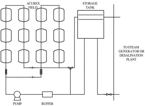
pipe where oil gets heated while circulating. Each collector uses the parabolic surface to focus the solar radiation onto the receiver tube, which is placed in the focal line of the parabola. The heat-absorbing oil is pumped through the receiver tube, causing the oil to collect heat, which is transferred through the receiver tube walls. The thermal energy developed by the field is pumped to the top of the thermal storage tank, whereupon the oil from the top of the storage tank can be fed to a power-generating system, a desalination plant, detoxi fi-cation plant or to an oil-cooling system if needed. The oil outlet from the storage tank to the field is at the bottom of the storage tank.
For the initial startup of the plant, the system is pro -vided with a three-way valve, which allows the oil to be circulated in the field until the outlet oil tempera ture is adequate to enter the storage tank. The oil pump, which pumps the oil from the storage tank, through the collector tubes and into the top of the storage tank is located at the field inlet, Fig. 1. To ensure that the collectors give optimum solar absorption, every collector row has a sun tracking system fitted to it.
A data acquisition system for the plant provides the following data: the solar intensity, inlet temperature to the field, outlet temperature of each loop and two other outlet temperatures between the field and storage tank, the current oil pump flow and requested value, and the tracking status of the collectors. The plant can generate 1.2 MW of peak power with beam solar radiation of 900 W m-2. The oil-storage tank has a capacity of 140 m3, which allows for storage of 2.3 thermal MWh for an inlet oil temperature of 210 oC and an outlet temperature of 290 oC.
The operation limits for the oil pump are between 2.0 and 10.0 litres per second. The minimum value is there for safety and to reduce the risk of the oil being decom-posed, which happens when the oil temperature exceeds 305oC. The consequence of exceeding the maximum oil temperature is that all the oil may have to be changed, leading to plant down time and loss of power generation. Another important restricting element in this system is the difference between the field’s inlet and outlet oil temperatures. A suitable, or normal, difference is around or less than 70 oC. If the difference is higher than 100 oC, then there is a significant risk of causing oil leakage due to high oil pressure in the pipe system.
A control system for this plant has the objective of maintaining the outlet temperature (in this case the average outlet temperature of all the parallel loops) at a desired level in spite of disturbances like solar irradiation (clouds and atmospheric phenomena), mirror reflectivity and inlet oil temperature. The oil flow rate is manipulated by the control system through commands to the pump. It should be noted that the primary energy source, solar radiation, could not be manipulated. The performance measures of the control system are to keep the oil outlet temperature close to its set point, and to avoid oscillations in the oil pump flow rate.
ACUREX FIELD
STORAGE TANK
PUMP BUFFER
TO STEAM GENERATOR OR
[image:2.596.306.547.83.259.2]DESALINATION PLANT
Fig. 1. Schematic representation of the solar plant
3. THE FEEDFORWARD TERM
The outlet temperature of the plant is influenced by changes in system variables such as oil flow, solar radiation, fluid inlet temperature, mirrors reflectivity, ambient temperature, etc. From the control point of view, the manipulative variable is the oil flow command to the pump. If either of the other variables change this introduces a change in the system output unrelated to fluid flow, which is the control input signal. Since both solar radiation and inlet temperature can be measured, this problem can be eased, by introducing a feedforward term in series with the system, calculated from steady state relationships. This makes an adjustment to the oil flow input, aimed at eliminating the change in outlet temperature caused by the variations in solar radiation and inlet temperature.
The input signal to the feedforward term is the set point temperature demanded by the controller and the output signal is the flow command to the pump. The linearised model is based on partial derivatives of the change in outlet temperature ∆To with respect to changes ∆u, ∆I,
and ∆Tin.
in in
o T
T f I I f u u f
T ∆
∂ ∂ + ∆ ∂ ∂ + ∆ ∂ ∂ =
∆ (1)
A simple approach, which reduces the complexity of the model, (Camacho et al., 1992), bases the feedforward term directly on the steady state energy balance relation-ship:
(
T
o−
T
in)
u
=
0
.
7869
I
−
0
.
485
(
T
o−
151
.
5
)
−
80
.
7
(2)where the output of the serial element forms the demanded oil flow signal us, which is calculated from the
following expression:
in s
T
u
u
I
u
−
−
−
−
=
0
.
7869
0
.
485
(
151
.
5
)
80
.
7
(3)Fig. 2. The input data to be modelled.
The computer model calculates the feedforward controller in a more complex way, incorporating two loss functions X1 and X2 to take into account such geometric
and thermal variables as solar hour, julianne day, inlet oil temperature etc.
4. DATA MODELLING 4.1 Fuzzy Subtractive Clustering
The clustering tool (Matlab, 2002) was used to identify natural groupings of the input data, Fig. 2, to produce a concise representation of the system’s high nonlinear behaviour, and hence give an initial idea of the cluster radius and number of input membership functions required to best represent that data, Fig. 3.
The cluster radius was then used as an initial starting point for a fuzzy inference generation function (genfis2) that builds on the subtractive clustering function to generate a Sugeno-type Fuzzy Inference System (FIS) that models the system behaviour from the input training data. The model FIS was then tested with twenty five data points of testing/checking input data (different from the training data) using an evaluation function.
[image:3.596.57.291.84.256.2]Fig. 3. Optimum Clusters and Cluster Radius/Influence.
Fig. 4. Illustrates the poor performance of the input-tested model when compared with the output testing data.
The model evaluation was then compared with twenty five data points of testing/checking output data, which produced the results shown in Fig. 4.
4.2 ANFIS Optimisation
Due to the poor performance of the FIS, Fig. 4, an ANFIS was chosen to tune (adjust) its membership func-tions, using a combination of a backpropagation algori-thm and a least squares method. This allows the fuzzy system to learn from the input/output data set, adjusting the FIS parameters (parameter estimation) to reduce the error measure, defined as the sum of the squared difference between the actual and desired outputs.
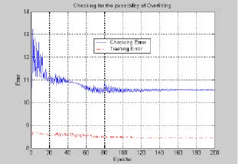
The FIS model was run initially under two hundred epochs of ANFIS training to create a new FIS model. This model was then checked for over-fitting of the fuzzy system to the training data by comparing the training input/output data with the checking input/output data (which in this case is the same as the testing data). Fig. 5 illustrates how a system can be over-fitted (the model’s ability to generalise the test data) when too many epochs are used. Here the training error settles at about the sixty-fifth epoch with no further improvement in the checking data error.
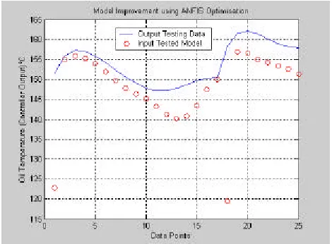
[image:3.596.57.286.552.738.2] [image:3.596.306.540.575.736.2]Fig. 6. Improved fit using ANFIS Optimisation.
The ANFIS was then run for sixty-five epochs to give the much improved results of Fig. 6. The 3-D Surface plot, Fig. 7, gives a good insight into the optimised FIS input/output relationships, while Fig. 8 shows the actual membership functions themselves. Here the main difference between the different shapes of the Mamdani-type of output membership functions and the Sugeno-type of FIS is well illustrated. The Sugeno always uses singleton spikes to determine its output membership functions, either crisply defined constants or in this case efficient linear first order equations of the form:
If x is A and y is B then z = p*x+q*y+r (4)
where A and B are the input fuzzy sets (antecedent) and p, q and r are the parameter constants of the first order linear equations that represent the output fuzzy set (singletons) of the Sugeno consequent. The values of these constants will be optimised further, by being considered as decis ion variables, to be randomly measured against a number of objective functions contained within a Multiobjective Genetic Algorithm (MOGA).
[image:4.596.308.539.84.260.2]Fig. 7. ANFIS Modelled Fuzzy Controller Input/Outputs.
Fig. 8. Input and Output Sugeno Membership Functions.
5. MOGA FINE TUNING
In an initial study by (Loebis, 2000), a fuzzy PI type controller, Fig. 9, was designed for better control of the solar plant’s low flow rates. This offered an improved overall performance compared with the standard PI controller. A MOGA was used to optimise the rule-base and membership functions for the Mamdani-type fuzzy controller against two performance criteria. Rise time, for each portion of the set point (due to each step input having a different step time, initial value and final value), and Covariance (for all portions), giving ten objective functions in all.
The fuzzy logic incremental controller (FLC) defined the error (e) as the difference between the plant’s output temperature (To) and the set point signal (Tr). The error
and its increment (∆e) were considered to be the inputs for the fuzzy controller and the output variable (∆u) was the increment to the control signal. A feedforward term was also added after the FLC to improve the dis turbance rejection caused by changes in the solar radiation.
Inference Engine
Fuzzify Defuzzify
Knowledge Base
Rule Base Date Base
Plant Feed-forward
Z- 1 Set Point
Temperature
Fuzzy Logic Controller
Z- 1
l Tin T
o uf u
∆e e
∆u -+
+
[image:4.596.322.521.546.737.2]-+
Fig. 10. GUI for Preference Articulation.
In the work presented here, the search space is reduced by allowing the fuzzy incremental controller to operate only in the higher nonlinear areas of the system, i.e. when the oil flow falls below 5 litres per second. This permits a wider choice of objectives, such as overshoot and settling time, because the set point change into this area has only one portion, i.e. it is more suited to the task-oriented nature of the fuzzy-type controller. Also having opti-mised input membership function sets, and an optiopti-mised output rule base, along with an efficient Sugeno FIS, gives the MOGA facility to quickly search for optimum output parameter sets.
Improvements to the work of (Schroder, 1999), on the decision support tool with the MOGA, are developed to improve the trade-off between solutions in the non-dominated set. This uses a novel technique of incorpora-ting conflict sensitivity or trade-off into the evolutionary process itself.
The MOGA uses the same Pareto-optimality criteria as developed by (Fonseca and Fleming, 1998), to determine fitness on the basis of non-dominance of the individuals. The criteria (including the four objectives) used to assess the performance of the fuzzy controllers are:
1. integral of the absolute value of the error 2. overshoot
3. rise-time 4. settling time 5. variance 6. oil flow rate
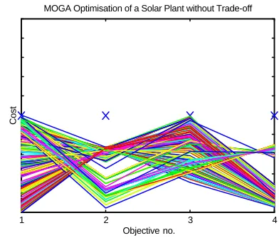
The ranges of the objective cost values are from -1 to 1, with the initial values of the goals scaled to zero, i.e. halfway, Fig. 11. A standard binary coded representation was employed with a chromosome length of 28 decision variables (12 for the parameters and 16 for the rules), each with 8 bit precision and a 20 bit decision variable bound. This compares well to the original controller, (Loebis, 2000) which required 60 decision variables. An Epanechnikov density kernel was used for the fitness sharing and mating limits. A rank fitness value of 2.22 was also used; hence exponential ranking was assumed indicating selective pressure.
6. ENHANCED DECISION SUPPORT
Here a novel enhancement to the MOGA decision support system is introduced, by using evolving tradeoff sensitivity information to automatically adjust the goal weighting. This is carried out to improve visualisation
1 2 3 4
Cost
Objective no.
[image:5.596.58.286.100.159.2]MOGA Optimisation of a Solar Plant without Trade-off
Fig. 11. Method of parallel coordinates.
and reduce the number of solutions in the non-dominated set, while at the same time maintaining the quality of those solutions.
As described in (Fonseca and Fleming, 1998), the population based nature of the standard GA makes it the ideal vehicle for the development of a Multiobjective Genetic Algorithm (MOGA) where several possibly competing objectives must be optimised simultaneously. Towards this end, goal and priority information are made available to the design objectives to make it possible to differentiate between some non-dominated solutions (best performers). These and other criteria form the basis of the decision support system that allows the decision maker to interactively control the final outcome of the simulation.
The method of goal and priority change (manually via a GUI) is called Progressive Preference Articulation, Fig. 10. The change of goal information allows the DM (Decision Maker) to investigate a smaller region of the search space or even to move on to a totally new region, which in turn affects the ranking of the population on that area of the search space. When priorities are assigned to a particular objective, zero priority corresponds to a standard objective to be optimised. A priority of 1 (minus 1 constraint in the GUI) defines a hard constraint, which has to be met, but not minimised once met. Higher priority values (minus 2, minus 3 etc.) define higher priority hard constraints. In a practical sense, the goals can be seen as the specifications of a design: an objective with zero priority might be percentage overshoot, whereas covariance for example could be treated as a constraint.
Methods for progressive articulation of preferences require that trade-off information be communicated to the decision maker in a form, which can be easily comprehended. When there are only two objectives, non-dominated solutions can be represented in objective space by plotting the first objective component against the second.
1 2 3 4 0
0 . 2 0 . 4 0 . 6 0 . 8 1
O b j e c t i v e N u m b e r
Cost
[image:6.596.61.254.81.234.2]M i n i m u m C o s t S o l u t i o n ( s ) f o r t h e S o l a r P l a n t
Fig. 12. Benchmark solution without using evolving trade-off.
integer index i to each objective and representing each non-dominated point by the line connecting the points (i,
f
ix
*
( )
), wheref
i*
represents a normalisation of fi to a
given interval, e.g., [0,1]. With such a representation, competing objectives with consecutive indices result in the crossing of lines, whereas lines that don’t cross indicate non-competing objectives, where the cost values
equate to
f
i*( )
x
and the objective numbers equate to f1-f4. Although the ordering of the objectives may be
automatically decided upon on the basis of some measure of competition (in order to maximise the competition between adjacent objectives, for example), being able to change this ordering interactively is also useful, and not difficult to implement.
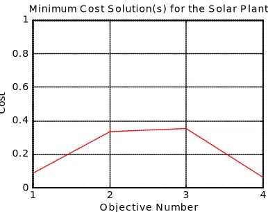
The development of the decision support system was initiated by computing the minimum cost solution. This will be used later as a benchmark or measure for quality of solution. The minimum cost solution was obtained by summing the objective costs for each individual in the non-dominated set, sorting them to obtain the minimum then extracting the minimum for display, see Fig. 12.
The graphical representation, shown in Fig. 11, and used by the multiobjective GUI tool, plots design objectives along the x-axis and the objective domain performance, within the environment of the problem, along the y-axis. Each line represents a single solution’s score against each objective. The displayed ranges of each objective are adjusted to leave the ‘×’ marks (in blue) representing the optimisation goals.
[image:6.596.349.482.86.214.2]Study of these trade-off graphs can lead to a greater understanding of the trade-offs inherent in the system. In Fig. 11, it is difficult to see the trade-off information clearly as the number of non-dominating solutions is too large. Therefore a tool has been developed by (Schroder, 1999) that allows a quantitative analysis of the amount of trade-off between objectives in such a graph, see Fig. 13.
This tool measures the amount of competition between objectives by computing the distance by which the lines cross as a percentage of the maximum distance that they could cross by. It uses a partitioning of the objective space to normalise with respect to the density of solutions
Percentage Trade-offs
1
2
3
4
1 2 3 4
(21)
(26)
(19)
(16)
3 5
13 9 4
3 9 7
5 4 7
13
Fig. 13. Percentage trade-offs (non-evolving), with the overall percentage trade-offs per objective in parenthesis.
so as not to allow highly populated parts of the objective space to artificially dominate the measure. The results of applying this tool to the graph of Fig. 11, are shown in Fig. 13.
The ranges upon which the trade-off figures are based are taken as the range between the maximum and minimum values of each objective. These represent the ‘true’ competition on the Pareto surface.
Each cell in the matrix of Fig. 13 represents the percentage trade-off between the objectives that represent its co-ordinates. The figures in parentheses on the diagonal are the sum of the trade-offs for that objective divided by the total number of objectives. This shows that the objective that caused the most amount of competition was objective two, which is reasonable when comparing it with the other objectives. The bar chart of Fig. 14 highlights the overall trade-off per objective for each objective on view. It gives an instant visual assessment of what is happening within the multi-criteria system being analysed.
A novel evolving goal weighting method is proposed in this work, that adjust the goals automatically in relation to trade-off information, which is only included if there are a minimum number of solutions in the non-dominated set. After each generation, this technique re-positions the goals to the initial maximum cost of each objective before it includes the trade-off information. The trade-off information tightens the goals on the objectives with
0 1 2 3 4 5
0 5 10 15 20 25 30
Total Percentage Non-Evolving Trade-offs
[image:6.596.327.510.589.732.2]Fig. 15. Goal weighting in relation to the average trade-off sensitivity.
1 2 3 4
Cost
Objective no. MOGA Optimisation of a Solar Plant without Trade-off
1 2 3 4
0 0.2 0.4 0.6 0.8 1
Objective Number
Cost
[image:7.596.310.521.107.231.2]Minimum Cost Solution(s) for the Solar Plant
Fig. 16. Results of the enhanced visualisation: without evolving trade-off (left) and with evolving trade-off (right).
Input 1 MF's (error) Input 2 MF's (∆error)
Output 1 MF's (∆control)
Rules 4
X X X
X
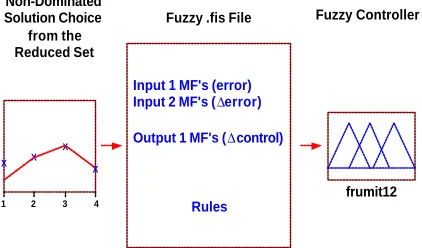
1 2 3 Non-Dominated Solution Choice
from the Reduced Set
Fuzzy .fis File Fuzzy Controller
frumit12
Fig. 17. Benchmark solution choice from the reduced set.
conflict sensitivity below the halfway or overall average objective sensitivity, and reduces the goals for the objectives that have conflict sensitivity above the overall average see Fig. 15.
7. RESULTS
[image:7.596.57.288.276.716.2]The enhanced decision support and visualisation im-proves the trade-off between the non-dominating solu-tions in the set while conserving the quality of the set, Fig. 16. The diagram shown in Fig. 17, illustrates how a
Table 1. Simulation without and with evolving trade-off
OBJECTIVES
O.shoot R.Time Err.Var. S.Time
Initial
Goals
5 20 10 315
Final
Goals
3.3 14.1 9.8 69.5
Min cost 0.3334 0.3513 0.4913 0.1130
Total Minimum Cost: Without: 1.2911 With: 1.2890
Number of Initial Individuals: 40
Total Percentage Trade-off: Without: 83% With: 30%
Number of Generations: 100
S tochastic Universal Sampling
Single Point Crossover Rate 0.7
Mutation Probability 0.007
Reinsertion 0.04
Minimum Number of Potential Solutions Found before
Trade-off Initiated: 5
Number of Near Optimum Solutions in the Non-Dominated Set: Without: 356 With: 351
ttt1 ttt2 ttt3 ttt4
mini maxi Half =
(maxi-mini)/2
midway = mini+half
1 2 3 4
Cost
Objective no. MOGA Optimisation of a Solar Plant with Trade-off
0 1 2 3 4 5
0 2 4 6 8 10
12 Total Percentage Evolving Trade-offs
1 2 3 4
0 0.2 0.4 0.6 0.8 1
Objective Number
Cost
Minimum Cost Solution(s) for the Solar Plant
0 1 2 3 4 5
0 5 10 15 20 25 30
[image:7.596.290.544.414.746.2]8.9 9 9.1 9.2 9.3 9.4 9.5 9.6 120
140 160
Solar Plant Start-up using Fuzzy Incremental Control
Time (24 hour clock)
Output Oil Temp. (C)
8.9 9 9.1 9.2 9.3 9.4 9.5 9.6 0
5
Time (24 hour clock)
Oil Flow (l/s)
8.9 9 9.1 9.2 9.3 9.4 9.5 9.6 200
400 600
Time (24 hour clock)
[image:8.596.66.270.83.269.2]Radiation (W/m2)
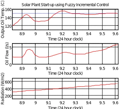
Fig. 18. Typical simulation results at plant start up time, for the fuzzy Incremental controller.
particular solution (in this case the benchmark) represents a particular fuzzy controller. The results of the conflict sensitivity between the solutions within the non-dominated set, before and after evolving trade-off is incorporated are shown in Table 1.
A typical response for the outlet oil temperature track-ing for the new improved fuzzy incremental controller at start up is shown in Fig. 18, along with the oil flow and radiation. In the figure, the single operating region facilitates the use of more design objectives. The design of the final controller is therefore a compromise that offers good performance across the highly non-linear operating range and also minimises the task-oriented nature of the set point tracking error.
7. CONCLUDING REMARKS
The design of an automatically tuned Sugeno-type incremental fuzzy controller for exclusive operation in high nonlinear regions:
• Reduced the rule base and search space, which in turn permitted the MOGA to produce a set of non-dominating solutions at a much faster rate.
• Improved control by allowing a wider choice of performance criteria.
• Increased the operating range at low oil flow rates, which allows the plant to function in environments where local solar radiation conditions have always been regarded as marginal.
The reduction in the size of fuzzy controllers is attractive because they are simpler to both understand and validate, and also easier to implement in hardware.
The work here also improved the visualisation techniques, required for a deeper understanding of the system. Allowing the trade-off, and hence goal information to evolve automatically gives the decision maker a solid foundation to work from, if further
alterations to the goal information are required manually, in order to arrive at the best non-dominating solution, for the optimal tuning of the fuzzy controller.
A benchmark solution was provided as a way to check that the qu ality of the non-dominating set has been maintained. It also provides the decision maker with an overall standard minimum cost solution from the non-dominated set.
ACKNOWLEDGEMENTS
R. Stirrup wishes to acknowledge the support of the UK Engineering and Physical Sciences Research Council.
REFERENCES
Camacho, E. F., Rubio, F. R. and Hughes, F. M. (1992). Self-tuning Control of a Solar Power Plant with a Distributed Collector Field. IEEE Control Systems Magazine, pp. 72-78.
Camacho, E. F., Berenguel, B. and Rubio, F. R. (1997). Advance Control of Solar Plants, 1st edn. pp. 23-45. Springer-Verlag, London.
Camacho, E. F., Berenguel, B. and Rubio, F. R. (1997). Advance Control of Solar Plants, 1st edn. pp. 47-56. Springer-Verlag, London.
Fonseca, C. M. and Fleming, P. J. (1998). Multiobjective Optimisation and Multiple Constraint Handling with Evolutionary Algorithms – Part 1: A Unified Formulation. IEEE Transactions Systems Management & Cybernetics. 28, pp. 26-37.
Johansen, T. A., Hunt, K. J. and Petersen, I. (2000). Gain-Scheduled Control of a Solar Power Plant. Control Engineering Practice. 8, pp. 1011-1022.
Ke, J. Y., Tang, K. S., Man, K. F. and Luk, P. C. K. (1998). Hierarchical Genetic Fuzzy Controller for a Solar Power Plant. ProceedingsIEEE International Symposium on Industrial Electronics, 7-10 July, Pretoria, South Africa, Vol. 2, pp. 584-588.
Loebis, D. (2000). Fuzzy Logic Control of a Solar Power Plant. Masters Dissertation. University of Sheffield, U.K. Malki, A. and Chen, G. (1994). New Design and Stability Analysis of Fuzzy Proportional-Derivative Control Systems. IEEE Transactions on Fuzzy Systems, 2, pp. 245-254.
Matlab Release R13 (2002), Fuzzy Logic Toolbox Documentation, The MathWorks, Inc.
Schroder, P. (1999). Controller Design Using Genetic Algorithms. In: Multivariate Control of Active Magnetic Bearings. PhD Thesis , University of Sheffield, U.K. pp. 20-39.