Copyright2001 by the Genetics Society of America
RNA Sequence Evolution With Secondary Structure Constraints: Comparison
of Substitution Rate Models Using Maximum-Likelihood Methods
Nicholas J. Savill,
1David C. Hoyle and Paul G. Higgs
School of Biological Sciences, University of Manchester, Manchester M13 9PT, United Kingdom Manuscript received July 17, 2000
Accepted for publication September 11, 2000
ABSTRACT
We test models for the evolution of helical regions of RNA sequences, where the base pairing constraint leads to correlated compensatory substitutions occurring on either side of the pair. These models are of three types: 6-state models include only the four Watson-Crick pairs plus GU and UG; 7-state models include a single mismatch state that combines all of the 10 possible mismatches; 16-state models treat all mismatch states separately. We analyzed a set of eubacterial ribosomal RNA sequences with a well-established phylogenetic tree structure. For each model, the maximum-likelihood values of the parameters were obtained. The models were compared using the Akaike information criterion, the likelihood-ratio test, and Cox’s test. With a high significance level, models that permit a nonzero rate of double substitutions performed better than those that assume zero double substitution rate. Some models assume symmetry between GC and CG, between AU and UA, and between GU and UG. Models that relaxed this symmetry assumption performed slightly better, but the tests did not all agree on the significance level. The most general time-reversible model significantly outperformed any of the simplifications. We consider the relative merits of all these models for molecular phylogenetics.
T
HERE are several classes of RNA molecules where in the helical regions of tRNA see Figure 1 of Higgs sequences are available over a wide range of species (1998).and where multiple sequence alignments are well estab- The mathematical theory of compensatory mutations lished,e.g., transfer RNA, 5S ribosomal RNA, small and was first discussed byKimura(1985), who showed that large subunit ribosomal RNA, and ribonuclease P RNA. compensatory changes can occur rapidly if the two sites Secondary structure is strongly conserved over long time are closely linked. The theory was developed byIizuka periods, indicating that selection is acting to maintain andTakefu(1996) and was studied specifically in the a structure that is essential for the function of these context of RNA helices byStephan(1996). These arti-molecules. The helical regions of the molecule are often cles treat mutation as irreversible and calculate the time quite variable in sequence. This shows that the precise until fixation of the double mutant as a function of the sequence of bases within the helical regions is of rela- mutation rate, the population size, and the strength tively little importance as long as the positioning of of selection against the intermediate (single mutant). these regions within the secondary structure is correct. Higgs(1998) has considered the same problem in the The mode of evolution within the helical regions is case of reversible mutations and has calculated fre-via pairs of compensatory neutral mutations;i.e., a muta- quency distributions for the different possible paired tion on one side of a pair disrupts the structure and is states.
slightly deleterious, but a second mutation of the other RNA sequences are often used in constructing molec-side of the pair restores the pairing ability. Compensa- ular phylogenies (e.g.,OlsenandWoese1993). If the tory pair changes form the basis of the comparative phylogenies are constructed using the helical regions method for deducing RNA secondary structures (Woese of RNA molecules then an understanding of the way in andPace1993;Gutell1996) and have also been the which these parts of the sequences evolve is important subject of several evolutionary studies (Wheeler and if reliable estimates of distances are to be obtained. Honeycutt 1988; Rousset et al. 1991; Vawter and Typically Markov models are used to represent the sub-Brown1993;Gatesyet al.1994;Kirbyet al.1995). For stitution process in the sequences. With 16 possible pairs an illustrative example of the degree of variability seen that can be formed with four bases a 16-state Markov
model, with a 16 ⫻16 rate matrix to describe relative rates from one state to another, is needed to study the
Corresponding author:Paul G. Higgs, School of Biological Sciences, evolution of the helical regions of RNAs. Models of University of Manchester, Oxford Rd., Manchester M13 9PT, United
this type have been proposed byScho¨ niger andvon Kingdom. E-mail: [email protected]
Haeseler(1994),Muse(1995), andRzhetsky(1995). 1Present address:Department of Mathematics, Heriot-Watt University,
Edinburgh EH14 4AS, United Kingdom. However, only the 6 matching pairs AU, GU, GC, UA,
UG, and CG occur frequently in helices, whereas the to and from mismatch states with any accuracy. Hence it is not cleara priori whether 16-state models give any other 10, so-called mismatch, pairs occur rarely,
presum-ably because they are deleterious mutations that destabi- advantage.
A third important issue is whether double substitu-lize the secondary structure. Since the mismatch states
are rare, it is reasonable to consider 6-state models that tions should be permitted in the rate matrix. It is fre-quently observed that pairs of closely related species allow only the 6 matching pairs, as was done byTillier
(1994) andTillierandCollins(1995). A third alter- differ by a pair of compensatory substitutions;e.g., a GC in one species is replaced by an AU in the other. Since native, rather than ignore mismatches completely, is to
group all the 10 mismatch (MM) pairs together into a mutation rates are very low in real organisms it is un-likely that these two changes occurred in a single organ-single state. This gives a 7-state model (Tillier and
Collins1998;Higgs2000). ism in a single generation. There were presumably some individuals with single mutant genotypes (in this case There is now a large variety of slightly different
mod-els. The principle aim of this article is to compare these probably GU) at some point in time. From the popula-tion genetics viewpoint the compensatory change can alternatives to see which is best able to describe real
sequence data. Some of these models involve a relatively happen in two ways. The first is by fixation of the slightly deleterious mutation (i.e., GU sequences rise to a high small number of parameters and make assumptions
about the symmetry of the rate matrix. This allows ana- frequency in the population) followed by fixation of the second mutation, which is now slightly advantageous lytical solution of the rate equations in several cases.
More complex models are straightforward to construct. (i.e., AU sequences arise and replace the GU se-quences). The second method is by the compensatory Increasing the complexity of a model will, in general,
improve the quality of the fit to the data. However, very substitution mechanism discussed by Kimura (1985), Stephan(1996), andHiggs(1998). In this case, slightly large numbers of parameters are sometimes not justified
because the extra parameters simply fit noise in the data deleterious single mutant sequences are created contin-ually by recurrent mutations, but their frequency is kept rather than any underlying trends. We therefore require
statistical techniques for this model selection process. very low by selection. If one of these sequences under-goes a second mutation this can create a sequence that Comparison of models of differing complexity has been
carried out for models of single nucleotide substitution is almost neutral with respect to the majority of the population. For example, GC sequences are in the ma-byYang et al.(1994), and here we carry out a similar
comparison for paired-site models. We analyze a set of jority, GU sequences are created in very small numbers, and one of these mutates to an AU. The neutral variant ribosomal RNA sequences using 18 different models.
For each model we obtain the maximum-likelihood solu- can then sometimes replace the original dominant vari-ant due to drift in gene frequencies. In this example tion for the frequency of the states, the rate matrix, and
the branch lengths of an example phylogenetic tree. the consensus sequence would change from GC to AU in a single step, and the GU sequences would remain Statistical tests are then used to compare the
maximum-likelihood values of the different models. as a minor variant throughout.
In phylogenetic studies, there is usually only one se-The most important issues to be considered when
comparing models are introduced at this point. First, quence available for each species, and there is no infor-mation available on minor sequence variants that might we might expect that the frequency of GC pairs should
be equal to that of CG, that the frequency of GU should exist in the population. The substitution rates therefore represent changes in the consensus sequence of the be equal to that of UG, and that the frequency of AU
should be equal to that of UA. We refer to this as “base population and do not represent rates of mutation in individual copies of a gene. Thus it is perfectly reason-pair reversal symmetry.” We wish to determine whether
models that allow arbitrary base pair frequencies fit the able to allow double substitutions in the rate matrix, even though double mutations in single genes probably data significantly better than models that assume base
pair reversal symmetry. Note that the first-mentioned almost never occur.Tillier andCollins (1998) and Higgs(2000) have used models that allow double sub-base in the pair is the one closer to the 5⬘end of the
molecule. Thus, for example, it is possible to unambigu- stitutions and find that the observed values of double substitution rates appear to be high. In this article we ously distinguish a GC from a CG pair by this rule, and
the equivalence of GC and CG pairs does not follow as use likelihood methods to determine if models that permit double substitutions fit the data significantly bet-a trivibet-al point.
Second, we wish to determine how to treat mis- ter than models that disallow double substitutions. matches. The 6- and 7-state models clearly throw away
information by ignoring mismatches or by treating them
MATERIALS AND METHODS in a simplified way. However, since the mismatch states
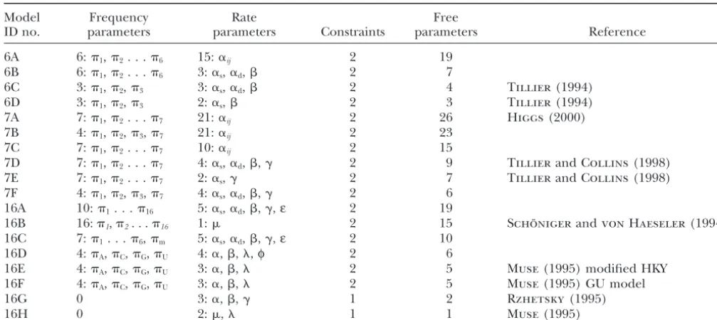
TABLE 1
Definitions of models
Model Frequency Rate Free
ID no. parameters parameters Constraints parameters Reference
6A 6:1,2. . .6 15:␣ij 2 19
6B 6:1,2. . .6 3:␣s,␣d, 2 7
6C 3:1,2,3 3:␣s,␣d, 2 4 Tillier(1994)
6D 3:1,2,3 2:␣s, 2 3 Tillier(1994)
7A 7:1,2. . .7 21:␣ij 2 26 Higgs(2000)
7B 4:1,2,3,7 21:␣ij 2 23
7C 7:1,2. . .7 10:␣ij 2 15
7D 7:1,2. . .7 4:␣s,␣d,,␥ 2 9 TillierandCollins(1998)
7E 7:1,2. . .7 2:␣s,␥ 2 7 TillierandCollins(1998)
7F 4:1,2,3,7 4:␣s,␣d,,␥ 2 6
16A 10:1. . .16 5:␣s,␣d,,␥,ε 2 19
16B 16:1,2. . .16 1: 2 15 Scho¨ nigerandvon Haeseler(1994)
16C 7:1. . .6,m 5:␣s,␣d,,␥,ε 2 10
16D 4:A,C,G,U 4:␣,,,φ 2 6
16E 4:A,C,G,U 3:␣,, 2 5 Muse(1995) modified HKY
16F 4:A,C,G,U 3:␣,, 2 5 Muse(1995) GU model
16G 0 3:␣,,␥ 1 2 Rzhetsky(1995)
16H 0 2:, 1 1 Muse(1995)
treatment of rate matrices has been developed in the context parameters minus the number of constraints. The constraints are Equation 4, for all models, and Equation 3, where appro-of single site models (see, for example,LiandGu 1996;Li
1997; Waddell and Steel1997). The rate equations used priate. The models are assigned identification codes A, B, C, etc. in order of decreasing numbers of free parameters. In all here are equivalent to those used for single site models, with
the exception that the number of states is 6, 7, or 16, instead the models, states 1–6 refer to the principal paired states in the following order: AU, GU, GC, UA, UG, CG. In 7-state of 4. The probabilityPij(t) that a base pair is in statejat time
tgiven that its ancestor was in stateiat time zero satisfies models, state 7 is MM. In 16-state models, states 7–16 refer to the 10 possible mismatch states in alphabetical order.
A general reversible model is the most general matrix of a dPij
dt ⫽
兺
kPikrkj. (1)
given number of states that satisfies Equation 5 (LiandGu
1996;WaddellandSteel1997). The most general reversible The diagonal elements of the matrix must satisfy
7-state model, labeled 7A, has 26 free parameters and is shown in Figure 1. This model was used by Higgs(2000), but has rii⫽ ⫺
兺
j⬆i
rij (2)
not previously been used with maximum-likelihood methods. Since this model has many parameters we wish to consider to conserve probability, and this constraint is included in the
whether simpler models will fit the data equally well. One definition of the models. At large timesPij(t) tends toj, the
natural simplification to make is to impose base pair reversal equilibrium frequency of statej, irrespective of the initial state
symmetry on model 7A by setting4⫽ 1,5⫽ 2, and6⫽
i.In some models the equilibrium frequencies are parameters
3. This gives model 7B. Another possible simplification is to
of the model; hence when fitting data we need to apply the
set all the␣parameters corresponding to double substitutions constraint
to zero, giving model 7C. Changes to and from the MM state
兺
i
i⫽1. (3) are treated as single substitutions and are not set to zero in 7C.TillierandCollins (1998) have also defined a 7-state model, here called 7D, and shown in Figure 1. This has 7 In other models, the frequencies are defined as functions of
frequency parameters and allows double substitutions. The other parameters, in which case constraint (3) applies
auto-many independent␣ijparameters in 7A are simplified to just 4: matically. When comparing models it is useful to have a
com-␣scontrols the single substitution rate,␣dcontrols the double
mon time scale. We choose the time scale so that an average
substitution rate,controls the double transversion rate, and of one substitution event per base pair happens in 1 time unit,
␥controls substitutions to and from the mismatch state. Fol-hence the constraint
lowing the usual convention, we define a transition as a
substi-兺
i i
兺
j⬆i
rij⫽1. (4) tution from one purine to another, or one pyrimidine to another, and a transversion as a substitution from a purine This constraint can be imposed by multiplication of all ele- to a pyrimidine or vice versa.
ments of the matrix by a constant factor. In addition, all the The three models 7B, 7C, and 7D arenestedin model 7A; models considered here are time reversible;i.e., they satisfy i.e., the simpler models are special cases of the more general model obtained by setting some parameters equal or some irij⫽ jrji. (5)
parameters to zero. Further simplifications of these models are possible. If the double substitutions are set to zero in 7D, Table 1 shows the models tested and summarizes the
param-we obtain 7E. If base pair reversal symmetry is imposed on eters involved. The number of free parameters in a model is
Figure 1.—Definition of the rate matrix for models 7A and 7D.
is shown in Figure 2, where an arrow indicates that the model
Figure2.—Relationships between the three groups of mod-at the head of the arrow is nested in the model mod-at the tail.
els. Each of the solid arrows indicates that the model at the The 6-state models are similar to the 7-state models, except
head of the arrow is nested within the model at the tail. that they lack the MM state. Model 6A is the general reversible
Statistical tests are made for each pair of models related in 6-state model. Models 6B and 6C are obtained by eliminating
this way. The dashed arrow indicates that a statistical test is the MM state from models 7D and 7F, respectively. Model 6D
made between the models that does not require the models is obtained by setting double transitions to zero in 6C. These
to be nested. 6-state models form a simple nested series, as shown in Figure
2. Models 6C and 6D were originally proposed by Tillier
(1994).
Muse(1995) proposed three models. The simplest, 16H, In principle we could define a general reversible 16-state
has only one free parameter after scaling the time. The second model with 134 free parameters; however, we do not believe
model, 16E, was termed the “modified Hasegawa-Kishino-Yano such a complex model would be practical, and we have not
(HKY) model” as it has several features in common with the attempted this. To facilitate comparison between the 6- and
model ofHasegawaet al.(1985) for single site evolution. It 7-state models and the 16-state models we have introduced
distinguishes between transition and transversion rates and models 16A and 16C, which are similar in spirit to model 7D.
allows the frequencies of the four bases to differ. The third The full matrix for 16A is shown in Figure 3. There are 16
model, 16F, is similar to 16E, but differs in its treatment of frequency parameters for the 16 states. The rate parameters
GU and UG pairs. In 16E, GU and UG pairs behave exactly for the 6 principal states are the same as those in 7D. Rates
as mismatches, whereas in 16F they behave exactly as Watson-of single substitutions to and from mismatch states are
con-Crick pairs. In natural RNA sequences, GU and UG frequen-trolled by a parameter ␥, and rates of single substitutions
cies are considerably lower than the Watson-Crick states, but between mismatch states are controlled by a parameter ε.
considerably greater than the mismatch states. We have there-Model 16C further simplifies the treatment of mismatches
fore introduced a model 16D by adding an extra parameter by setting the frequencies of all 10 mismatches to a single
φ that enables the GU and UG pairs to have intermediate parameterm. Models 16A and 16C are the only 16-state
mod-frequencies. The full rate matrix for 16D is given in Figure els that allow a nonzero rate of double substitutions.
4. The equilibrium frequencyXYof a base pairXYis related In the model proposed byScho¨ nigerandvon Haeseler
to the frequencies of the two basesXandYbyXY⫽ XY2 (1994), the rates are defined asrij⫽ jif statesiandjdiffer
ifXandYform a Watson-Crick pair;XY⫽ XYφ2ifXand by a single substitution and zero otherwise. To apply Equation
Yare GU or UG;XY⫽ XY ifXandYform a mismatch. 4 we introduce an extra factor, so thatrij⫽ j, and then
The constantis determined by scaleto satisfy (4). This model, termed 16B, is identical to
that ofScho¨ nigerandvon Haeseler(1994), except for the 1/ ⫽2(2⫺1)(
AU⫹ GC)⫹2(φ2⫺1)GU⫹1. (6)
timescale. Since the timescale does not affect the
Figure3.—Definition of the rate matrix for model 16A.
bases have equal frequency and there is no difference between confirmed the tree topology using the dnaml and dnapars programs in the Phylip package (Felsenstein1995). transitions and transversions.
Rzhetsky(1995) also proposed a 16-state model, labeled The sequence alignments and the positions of the conserved secondary structures given byvan de Peeret al.(1998) were 16G. This model is a simplification of 16B, which is obtained
by setting the frequencies of the four Watson-Crick states to taken to be correct. This analysis uses only the paired regions of the sequence and ignores the loop regions. We have pre-be equal, the frequencies of GU and UG to pre-be equal, and the
frequencies of the mismatch states to be equal. The relation- viously analyzed the frequencies of base pairs in a set of over 400 sequences from the same database that includes a repre-ship between the 16-state models is shown in Figure 2.
The maximum-likelihood calculation:A set of eubacterial sentative from each genus of eubacteria (Higgs 2000). In
general it is found that GU and UG pairs have low frequencies, small subunit ribosomal RNA sequences was obtained from
the rRNA database (van de Peeret al.1998). The object is not as would be expected if they are slightly deleterious. However, a small fraction of the paired sites have a GU or UG pair in to test the tree topology but to test the evolutionary models;
therefore we chose five species for which the rRNA phylogeny a majority of sequences. This suggests that these pairs are positively selected when they occur at particular points in the is well established.Bacillus subtilisis a member of the
gram-positive bacteria and is an outgroup to the remaining four structure (see alsoRoussetet al.1991;Gautheretet al.1995). Such sites violate the assumptions of all the models discussed in proteobacteria.Rhodomicrobium vannieliiandSphingomonas
cap-sulataare examples of the alpha proteobacteria subdivision, this article, which treat GU and UG pairs as slightly deleterious alternatives to Watson-Crick pairs. For this reason, paired sites whileEscherichia coliandPseudomonas aeruginosaare examples
of the gamma proteobacteria subdivision. The tree is shown at which the observed GU frequency or UG frequency in the full set of sequences was⬎50% were excluded from the analy-in Figure 5 analy-in unrooted form. This tree is the one given
by both the National Center for Biotechnology Information sis carried out in this article. The analysis was carried out on 296 pairs (i.e., 592 sites) that satisfied these criteria. The effect taxonomy browser (LeipeandSoussov1995) and the
Ribo-somal Database Project (Maidaket al.1999). In addition we of inclusionvs.exclusion of these pairs is discussed in more
to the rates and frequencies were discarded. Checks were made that the algorithm converged to the same optimal pa-rameter values from different starting points. For some of the models we also checked the results from our optimization algorithm against results obtained using a simple simulated annealing algorithm (Kirkpatricket al.1983;Kirkpatrick
1984) to locate the maximum-likelihood values of times and model parameters. No significant differences were found be-tween the results of our hill climbing algorithm and the simu-lated annealing algorithm, indicating that the hill climbing algorithm was indeed adequate for the task. For each set of
Figure 5.—The phylogenetic tree used for testing the
rates, the optimum times were calculated to the nearest 0.001 models.
unit for the 6- and 7-state models, and to the nearest 0.01 unit for the 16-state models, since these required greater computer time to calculate.
detail byHiggs(2000), using a different method of sequence
Statistical tests:Having estimated the maximum-likelihood
analysis. Elimination of these unusual pairs does not favor any
parameter set for each of the models, we have a likelihood one model over any other and therefore does not influence
valueLfor each model, which is the likelihood of the given the model selection criteria in this article.
sequences on the given tree assuming the optimized values When testing the models we assumed that the topology of
of the parameters. In general a largerLindicates a better fit the tree was fixed, but not the branch lengths. For each model
of the model to the data; however, in choosing between models we obtained the parameter set that maximized the likelihood
it is not sufficient to select the one with the highestL.There of observation of the given sequences on the given tree.
Meth-is a tendency for models with more parameters to give higher ods of calculating the likelihood are discussed byFelsenstein
Lvalues. In fact, in cases where models are nested, the one (1981),Swofford et al.(1996), andLi(1997). In our case,
with the larger number of parameters will always give the the adjustable parameters consist of the parameters defining
higherL.However, the use of additional parameters is some-the model (as defined in some-the previous section and in Table
times not justified statistically. 1) and the seven branch lengths in the unrooted tree (as
A criterion often used to compare models is the Akaike shown in Figure 5).
information criterion (AIC;Linhart and Zucchini 1986), When using the six-state models, a decision had to be made
defined as AIC⫽ ⫺lnL ⫹ number of free parameters (or as to what to do with the mismatch states that do actually
sometimes as twice this). Theory suggests that the model with occur in the real sequences. Positions where there are many
the lowest AIC is to be preferred. The AIC thus penalizes mismatches do not count as paired sites in the consensus
models with too many parameters. secondary structure in the database, and therefore these sites
The likelihood-ratio test (LRT) makes a direct comparison are not considered. However, there remain sporadic
mis-between two modelsH0andH1, whereH0is the simpler model
matches occurring rather randomly throughout the sequence
nested within the more general modelH1. IfL0is the likelihood
alignment in positions where almost all the other sequences
of the data according toH0, andL1is the likelihood of the
are properly paired. We did not wish to discard the complete
data according toH1, then the LRT proceeds by calculating
column of data from the sequence alignment, simply because
the logarithm of the likelihood ratio:␦ ⫽ln(L1/L0). Even if
a single sequence in the set had a mismatch at that position.
H0is perfectly valid␦will still be positive, sinceH1has a larger
Therefore, any mismatch states that occurred were treated as
number of parameters with which to fit the data. Theory shows being the same as the Watson-Crick pair that has the same 5⬘
(Linhart andZucchini1986) that if the simpler model is base;i.e., AA, AC, and AG are treated as AU, while GA and
true then 2␦will be distributed according to a2distribution
GG are treated as GC, etc. In this way the mismatch states are
with the number of degrees of freedom equal to the difference distributed roughly equally between the four main states.
in the number of parameters between the two models. As a The maximum-likelihood values of the parameters for each
significance test we can calculate the probability Pthat 2␦ model were calculated as follows. An initial estimate of the
from the 2 distribution will be greater than the observed
state frequencies was obtained by measuring the average
fre-value of 2␦. A small Pindicates that the observed result is quencies in the data. The initial rate matrix was estimated by
unlikely to occur by chance ifH0is an adequate model, and
calculating the frequency of changes of states between pairs
hence thatH1is a significantly better fit to the data. A large
of sequences. The individual rates were estimated by
calculat-Pindicates that introduction of the extra parameters inH1
ing the number of differences of each type between sequence
does not significantly improve the fit given byH0.
pairs and normalizing using Equation 4. The rates were then
The proofs of the AIC and LRT rely on the asymptotic averaged over all pairs of sequences. The initial times were
assumption, i.e., that there is a very large amount of data. estimated by finding the maximum-likelihood divergence time
For the case of phylogenetic methods this means that the for pairs of sequences given the initial estimation of the rate
sequences should be extremely long.Goldman (1993) has matrix.
cast doubt on the validity of these asymptotic tests for analysis Once initial values of the parameters had been estimated
of biological sequences of realistic length and has proposed an iterative algorithm was used to calculate the maximum
that Cox’s test should be used instead. This test (Cox1962) likelihood of the data. The algorithm was iterated until the
works by calculating␦for two models as in the LRT. Although maximum likelihood converged (typically 1000–2000
itera-the distribution of␦cannot be calculated analytically if the tions but this depends on the model being studied). At each
asymptotic results do not apply, it can still be simulated numer-iteration a small random change was made to a single rate
ically. After fitting the real data and calculating the maximum-parameter and a single frequency maximum-parameter.Pij(t) was solved
likelihood parameters according to both models, a large num-by numerical integration of Equation 1 and the
maximum-ber of sets (typically 100) of simulated sequences are generated likelihood values of the times were calculated by a hill climbing
using the modelH0. Each of the simulated sets is then refitted
method in time-space. If the new value of the maximum
likeli-using both models, and a histogram of␦values is obtained hood was greater than the best value found so far, the new
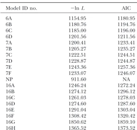
TABLE 2 three groups of models because the states are different, and the sequence data are treated in a different way.
Maximum-likelihood and AIC values
The more possible states there are, the smaller the likeli-hood of change between any two individual states.
Model ID no. ⫺lnL AIC
Hence models with more states have lower likelihoods
6A 1154.95 1180.95 and higher AICs, but this does not tell us anything about
6B 1180.76 1194.76
the relative merits of the three groups of models.
6C 1185.00 1196.00
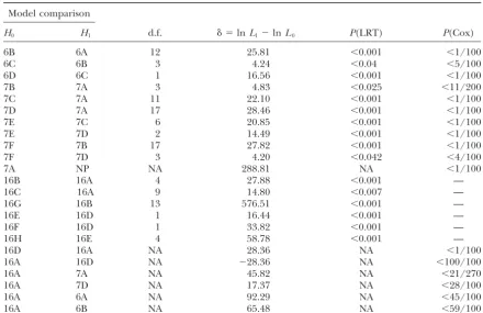
Table 3 shows the outcomes of the statistical tests
6D 1201.56 1211.56
between the model pairs. Tests are carried out for pairs
7A 1200.41 1233.41
7B 1205.27 1235.27 of models linked by arrows in Figure 2. The number of
7C 1222.51 1244.51 degrees of freedom (d.f.) for each test is also given. The
7D 1228.87 1244.87 significance values for the LRT areP values obtained
7E 1243.36 1257.36 from a 2 table. For all but two of the Cox tests, 100
7F 1233.07 1246.07
replicates were performed. In many cases there were
NP 911.60 NA
no simulated␦ values greater than the real value, and
16A 1246.24 1272.24
we quote this as a significance ofP⬍1/100. For cases
16B 1274.12 1296.12
16C 1261.03 1278.03 where there weren simulated values higher than the
16D 1274.60 1287.60 real value out ofmreplicates we have quotedP⬍(n⫹
16E 1291.04 1303.04 1)/m. Where the level of significanceP was small and
16F 1308.42 1320.42 the outcome of the Cox test critical in affecting our final
16G 1850.62 1859.10
choice of model, we have performed a larger number of
16H 1365.52 1373.52
replicates to reduce the expected error in the estimated
NA, not applicable. level of significance obtained from the Cox test. This
was the case for the comparison of 16A and 7A, where we performed 270 replicates, and for the comparison fraction of the simulated sets that have ␦ higher than the
of 7B and 7A, where we performed 200 replicates. observed value for the real data. This test is to be preferred
over the other two since it involves no assumptions on the We discuss the 6- and 7-state models together, since distribution of␦; however, it requires very much greater com- the conclusions are very similar. The question of puter time. In cases where the tree topology is not known, it whether base pair reversal symmetry is valid is addressed is usual to estimate the maximum-likelihood tree topology for
by the comparison 7B-7A in Table 3. The more general both the real data and each set of simulated data when doing
model gives a significantly better fit with P ⬍ 0.025 the Cox test. We did not do this. When fitting the simulated
data the tree topology was kept fixed while the branch lengths according to the LRT and a marginally significant better and rate parameters were varied, in the same way as was done fit withP⬍0.055 according to the Cox test. The distribu-for fitting the real data. As long as the same procedure is used tions are shown in Figure 6. Once again the more gen-for fitting the real and the simulated data, the statistical test
eral model has the lower AIC and consequently overall is valid.
we consider 7A to be a better model than 7B. The same The adequacy of the most general models cannot be tested
by comparison to any of the other models. However, they question is also addressed by the comparisons 7F-7D can be compared to a nonparametric (NP) model (Goldman and 6C-6B. In both these cases the more general model
1993). A position along the aligned sequences will exhibit a has the lower AIC, suggesting that we should not make combination C of states called a pattern. This pattern occurs
the assumption of base pair symmetry. However, the with a certain frequency in the aligned sequences. The
maxi-two tests for 7F-7D and 6C-6B giveP⫽4 or 5%, which mum-likelihood solution for the NP model takes the form
is only marginally significant. Higgs (2000) has also L⫽
兿
C
(NC/N)NC, (7)
observed that GC frequency is considerably higher than CG frequency in several large datasets of RNA se-whereNCis the number of occurrences of the patternC in
quences, but it is not clear what the cause of this could the aligned sequences. We carried out the Cox test for model
7Avs.the seven-state NP model. be. Thus, taken together, the results suggest that there may be some effect present that breaks the symmetry between these apparently equivalent states, but in ab-RESULTS
sence of a theory as to why this should happen, and in view of the borderline statistical significance, it is not The values of the log-likelihood and the AIC statistical
test as well as the optimal phylogenetic tree times for possible to rule out that the apparent loss of base pair reversal symmetry is a result of chance alone.
each model are shown in Table 2. Since the lowest AIC
is to be preferred, we see that the general reversible The comparison 7C-7A tests whether double substitu-tion rates may be set to zero. The answer is clearly no: 6-state model 6A is the best of the 6-state models, the
general reversible 7-state model is the best of the 7-state 7A is a better fit than 7C with very significantP values according to both pairwise tests. Also, the AIC is lower models, and model 16A is the best of the 16-state models.
TABLE 3
Likelihood-ratio and Cox’s tests
Model comparison
H0 H1 d.f. ␦ ⫽lnL1⫺lnL0 P(LRT) P(Cox)
6B 6A 12 25.81 ⬍0.001 ⬍1/100
6C 6B 3 4.24 ⬍0.04 ⬍5/100
6D 6C 1 16.56 ⬍0.001 ⬍1/100
7B 7A 3 4.83 ⬍0.025 ⬍11/200
7C 7A 11 22.10 ⬍0.001 ⬍1/100
7D 7A 17 28.46 ⬍0.001 ⬍1/100
7E 7C 6 20.85 ⬍0.001 ⬍1/100
7E 7D 2 14.49 ⬍0.001 ⬍1/100
7F 7B 17 27.82 ⬍0.001 ⬍1/100
7F 7D 3 4.20 ⬍0.042 ⬍4/100
7A NP NA 288.81 NA ⬍1/100
16B 16A 4 27.88 ⬍0.001 —
16C 16A 9 14.80 ⬍0.007 —
16G 16B 13 576.51 ⬍0.001 —
16E 16D 1 16.44 ⬍0.001 —
16F 16D 1 33.82 ⬍0.001 —
16H 16E 4 58.78 ⬍0.001 —
16D 16A NA 28.36 NA ⬍1/100
16A 16D NA ⫺28.36 NA ⬍100/100
16A 7A NA 45.82 NA ⬍21/270
16A 7D NA 17.37 NA ⬍28/100
16A 6A NA 92.29 NA ⬍45/100
16A 6B NA 65.48 NA ⬍59/100
NA, not applicable.
The histogram of ␦values from Cox’s test is shown in have assumed equal rates of substitution at each site. Relaxing this assumption may give better models but Figure 6, in comparison to the 1⁄
22 distribution
(ex-pected according to the LRT) and to the real value in also may increase the number of parameters to fit. Com-parison with the NP model is a very stringent test, and the data (denoted by an arrow). It can be seen that
the real value is completely outside the range of the it seems unlikely that any reasonably tractable model would ever pass the test when applied to real sequence distribution, hence P is very much ⬍1% and it would
require many more than 100 replicates to estimate a data. This test is rather unhelpful since it tends to reject models without proposing any better alternative. truePvalue. The question of zerovs. nonzero rates of
double substitutions is also addressed by the comparison One point that can be seen for all the results with the 6- and 7-state models is that the Cox test with numeri-of 7E-7D, in which the parameters␣dand are set to
zero, and 6D-6C in which␣dis set to zero (note that cal simulation of the␦distribution always gives very
simi-lar results to the much simpler LRT. The conclusion cannot be zero in the 6-state model, otherwise the states
are divided into two inaccessible subsets of three). In reached on significance is the same in every case, and the simulated distributions differ rather little (if at all) both these two comparisons the model with the nonzero
rates gives a much better fit (very lowPvalues) and also from the1⁄
22distributions assumed by the LRT.
There-fore it would seem that the LRT is an appropriate test gives a lower AIC.
Model 7D is of interest because it is the most complex for analysis of these sequences despite the original doubts that there may not be sufficient data to be in of the models for which an analytical solution is available
(Tillier and Collins 1998). Model 7D has 17 fewer the asymptotic regime. It was also found that the Cox test on the 16-state models was extremely slow (note that parameters than 7A, which gives it a large advantage on
the AIC test. Nevertheless, the general model has a much every comparison requires 200 runs of the maximum-likelihood program). For these two reasons we did not lower AIC. It can also be seen (Figure 6 and Table 3)
that 7A gives a highly significant improvement over 7D. perform a Cox test for every pair of 16-state models and decided to rely on the results of the LRT. The Cox Even though the general model 7A outperforms the
alternatives, comparison with the nonparametric model test was only performed for the 16D-16A and 16A-16D comparisons, for which the LRT is not valid because in Table 3 indicates that it is still not an adequate
Figure 6.—Distributions of␦for four of the pairwise comparisons between mod-els. The histograms indicate distributions simulated by the Cox test. The continuous dis-tributions in the first three graphs are 1⁄
22distributions.
Observed values of␦are indi-cated by arrows.
The two best 16-state models according to the AIC significantly better than 16D (P⬍0.01)]. The simulated distribution of␦values is shown in Figure 6, from which are 16A and 16C. These are the two models that have
nonzero rates of double substitution. The model of it can be seen that the majority of simulated values are negative; i.e., if 16D were the true model, then 16A Scho¨ niger andvon Haeseler (1994), 16B, is nested
in 16A (by setting␣d and to zero and ␣s ⫽ ␥ ⫽ ε). would usually not fit the data better than 16D. In
con-trast,␦ is positive for the real data, indicating that it is Model 16A is significantly better than 16B by the LRT
and the AIC. Model 16C also performs less well than better explained by 16A. This test can also be performed in the reverse direction by using 16A to simulate the 16A, although it is still better than any of the other
16-state models. In model 16C the frequencies of all the data. In this case ␦ is negative for the real data, and none of the simulated data give a␦as low as this (i.e., mismatch states are set equal to one another. This result
shows that there is a significant improvement in the P⬍ 100/100). Thus if 16A were the true model then it would be highly unlikely that the difference in likeli-likelihood if all the mismatch frequencies are allowed
to vary independently. hood between the two models would be as high as it is. From this point of view we can conclude that 16A is Of the two models 16E and 16F proposed by Muse
(1995), 16E is the better. We proposed model 16D as not an entirely adequate description of the real data. Nevertheless it is still better than any of the alternatives a generalization of both of these two to allow the LRT
to be performed. The comparisons 16E-16D and 16F- considered.
Through use of the Cox test we can compare the 16D by the LRT indicate that 16D is a significant
im-provement over both the others. The maximum-likeli- performance of models with differing numbers of states. We have performed Cox tests between the best models hood values of the parameters in 16D were ⫽13.41
andφ⫽ 2.93. The fact that φis closer to 1 than to in each class, i.e., between 16A and 7A, and between 16A and 6A. We have also compared 16A with 7D and indicates that the GU and UG pairs are closer in
behav-ior to the mismatch pairs than to Watson-Crick pairs 6B, since these two models have exactly the same form of the matrix for the principal states as 16A. The tests according to this model.
The AIC suggests that all three models 16D, 16E, and give P values between 7 and 59%;i.e., there is no evi-dence for rejecting 16A. The 7% value for the 16A-7A 16F perform less well than 16A and 16C. This cannot
be checked by the LRT because the models are not comparison is the smallest of these four values, which gives some degree of support to choosing 7A as the nested. We therefore performed a Cox test between
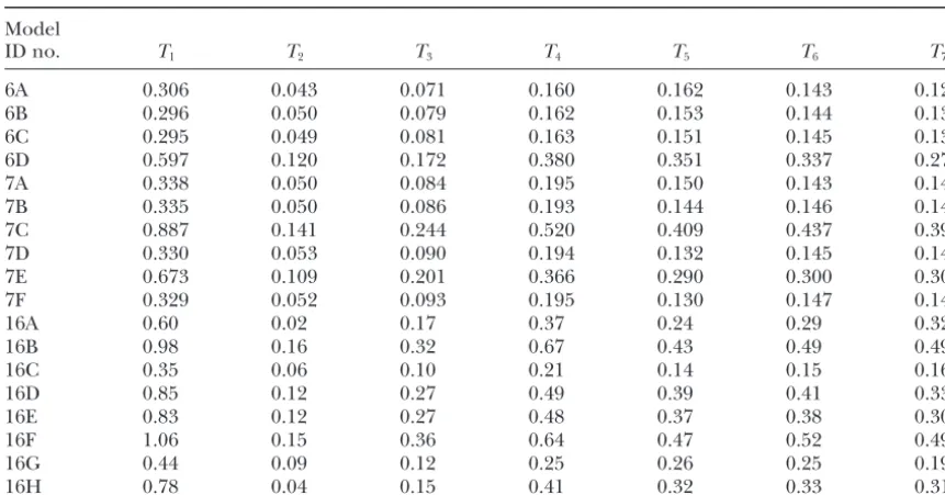
can-TABLE 4
Branch lengths
Model
ID no. T1 T2 T3 T4 T5 T6 T7
6A 0.306 0.043 0.071 0.160 0.162 0.143 0.126
6B 0.296 0.050 0.079 0.162 0.153 0.144 0.132
6C 0.295 0.049 0.081 0.163 0.151 0.145 0.130
6D 0.597 0.120 0.172 0.380 0.351 0.337 0.277
7A 0.338 0.050 0.084 0.195 0.150 0.143 0.144
7B 0.335 0.050 0.086 0.193 0.144 0.146 0.140
7C 0.887 0.141 0.244 0.520 0.409 0.437 0.390
7D 0.330 0.053 0.090 0.194 0.132 0.145 0.149
7E 0.673 0.109 0.201 0.366 0.290 0.300 0.303
7F 0.329 0.052 0.093 0.195 0.130 0.147 0.147
16A 0.60 0.02 0.17 0.37 0.24 0.29 0.32
16B 0.98 0.16 0.32 0.67 0.43 0.49 0.49
16C 0.35 0.06 0.10 0.21 0.14 0.15 0.16
16D 0.85 0.12 0.27 0.49 0.39 0.41 0.33
16E 0.83 0.12 0.27 0.48 0.37 0.38 0.30
16F 1.06 0.15 0.36 0.64 0.47 0.52 0.49
16G 0.44 0.09 0.12 0.25 0.26 0.25 0.19
16H 0.78 0.04 0.15 0.41 0.32 0.33 0.31
not be performed in the reverse direction. If 7-state wherever there have been compensatory changes this counts as two changes in state. In the other models a models are used to generate the data, then the data will
contain MM states that cannot be treated properly in double substitution usually occurs as a single step. The same effect shows up in the 7-state models, where the 16-state models or in 6-state models. If 6-state models
are used to generate the data, there will be no mismatch branch lengths are apparently much larger in models 7C and 7E where double substitution rates are zero. states of any kind, hence there will be no point in fitting
the simulated data to 7-state and 16-state models. Thus The times are also larger for 7-state models and corre-sponding 6-state models (e.g., 7A and 6A) because the we cannot reject 16A in favor of any of the other models,
but, equally, we cannot reject the others in favor of 16A. 7-state models count changes to and from mismatch states that are not counted in 6-state models. In terms These tests are therefore not very helpful in deciding
how many states to use. of relative branch lengths, however, there is not much difference between the 6- and 7-state models. It is the When choosing a rate model for molecular
phyloge-netics, it is not just the likelihood value that needs to relative values of the lengths that are most important, because the absolute values only have a meaning if a be taken into account, but also the speed of calculation.
Sixteen-state models require considerably more time for molecular clock calibration is used to assign times to the different branch points on the tree (which we have likelihood calculations; therefore, since we have been
unable to demonstrate a clear advantage for any of the not attempted with these data). For the 16-state models, there is considerable difference in the branch lengths 16-state models, we propose not to use them in our future
phylogenetic studies. Our preference is for model 7A, according to the different models. This is another rea-son why we prefer the 6- and 7-state models to the 16-from the results of the above tests, and model 7D, since
this is the best of the models that is analytically solvable. state models. The analytical solution again allows savings in computer
time in ML methods and easy calculations of pairwise
DISCUSSION distances for use in distance matrix methods.
TABLE 5
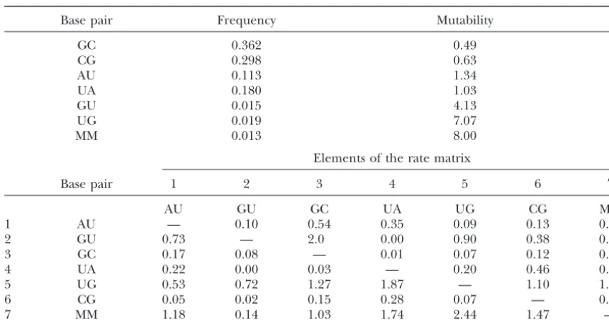
Maximum-likelihood values of the parameters in model 7A
Base pair Frequency Mutability
GC 0.362 0.49
CG 0.298 0.63
AU 0.113 1.34
UA 0.180 1.03
GU 0.015 4.13
UG 0.019 7.07
MM 0.013 8.00
Elements of the rate matrix
Base pair 1 2 3 4 5 6 7
AU GU GC UA UG CG MM
1 AU — 0.10 0.54 0.35 0.09 0.13 0.13
2 GU 0.73 — 2.0 0.00 0.90 0.38 0.12
3 GC 0.17 0.08 — 0.01 0.07 0.12 0.04
4 UA 0.22 0.00 0.03 — 0.20 0.46 0.12
5 UG 0.53 0.72 1.27 1.87 — 1.10 1.58
6 CG 0.05 0.02 0.15 0.28 0.07 — 0.06
7 MM 1.18 0.14 1.03 1.74 2.44 1.47 —
sequences used here, we compare these results to those the method given inHiggs(2000) efficiently uses infor-mation from very many sequences, even though it is less in the previous article. The complete
maximum-likeli-hood rate matrix for 7A is also shown in Table 5, to- rigorous than the ML method. We emphasize that the results obtained in this article support the conclusions gether with the maximum-likelihood values of the
fre-quencies and the mutabilities. The mutability of a state given in the previous article regarding the relative rates of different types of substitution and the influence of is the net rate of substitution from that state to all other
states (i.e., it is the negative of the element on the diago- thermodynamics on the substitution process.
The ranking order of the models given by the tests nal of the rate matrix). A mutability of 1.0 indicates
that the state changes at the average rate for the whole used here applies only to the particular set of sequences used and should therefore be treated with some caution. sequence.
It can be seen that GC and CG pairs have low mutabili- However, we believe that very similar selective effects are occurring in helical regions of many types of RNA, ties and high frequencies, that AU and UA pairs have
moderate frequencies and mutabilities, and that GU, as was discussed fully by Higgs (2000). Therefore we expect that the models that perform best in this analysis UG, and MM pairs have low frequencies and high
muta-bilities. The order of the base frequencies is the same will also generally be the best models for describing other RNAs with conserved structure. This will be tested as that of the thermodynamic stability of stacking
inter-actions. This shows that sequences are selected to in- in further work.
Although it is clear from the statistical analysis that crease the thermodynamic stability of the secondary
structure. It can also be seen that rates of double transi- general models such as 7A give significantly higher likeli-hoods than analytically tractable models like 7D, the tions are large;e.g., AU to GC and UA to CG are actually
higher than the rates of the single transitions AU to GU analysis does not say why this is. However, it is not diffi-cult to see why there should be a lack of symmetry in and UA to UG. This shows that the single-step
compen-satory mutation mechanism is occurring frequently in the rate matrix. First, real molecules may be subject to mutational bias, such that new bases do not arise with these sequences. The five sequences used here are a
subset of the rRNA-1 set used by Higgs (2000). The equal frequency. Second, there are many different selec-tive effects. As discussed above, we believe that double values of the parameters are close to those obtained for
the rRNA-1 set but not identical because of the method substitutions are occurring via a single-step compensa-tory mechanism. The rate at which this occurs is strongly of fitting the model to the data. The ML method used
here has the advantage of allowing rigorous statistical influenced by the fitness of the intermediate state. Dou-ble transitions between Watson-Crick pairs occur via GU tests, but is limited to a small number of sequences
because of the computer time required. We consider it and UG intermediates, whereas double transversions have to pass via true mismatches like GG or CC. True an open question which of these methods gives a more
the helix and therefore presumably a much lower fit- LITERATURE CITED
ness. This accounts for the slow rate of double transver- Cox, D. R., 1962 Further results on tests of families of alternate hypotheses. J. R. Stat. Soc. B24:406–424.
sions with respect to double transitions. The
thermody-Felsenstein, J.,1981 Evolutionary trees from DNA sequences: a namics of stacking interactions is far from symmetric
maximum likelihood approach. J. Mol. Evol.17:368–376. (see Higgs 2000 and references therein); i.e., not all Felsenstein, J.,1995 Phylip (Phylogeny Inference Package), version
3.5c. mismatches are equivalent. Also, interactions occur
be-Gatesy, J., C. Hayashi, R. DeSalleandE. Vrba,1994 Rate limits tween stacked pairs within a helix, not just between the for pairing and compensatory change: the mitochondrial ribo-two bases in a pair. Therefore, we might expect to see somal DNA of antelopes. Evolution48:188–196.
Gautheret, D., D. KoningsandR. R. Gutell,1995 GU base pair-further correlations in substitutions involving more than
ing motifs in ribosomal RNA. RNA1:807–814.
just two sites. In view of all these effects we do not find Goldman, N.,1993 Statistical tests of models of DNA substitution. it surprising that the rate matrix does not have a simple J. Mol. Evol.36:182–198.
Gutell, R. R.,1996 Comparative sequence analysis and the struc-symmetry.
ture of 16S and 23S RNA, pp. 15–27 inRibosomal RNA: Structure,
We became aware of two other models for RNA helix Evolution, Processing, and Function in Protein Biosynthesis, edited by evolution after the analysis of the models in this article R. A. ZimmermannandA. E. Dahlberg.CRC Press, Boca Raton,
FL. was almost complete.M. Scho¨ nigerandA. von
Haese-Hasegawa, M., H. KishinoandT. Yano,1985 Dating of the human-ler (personal communication) have considered an- ape splitting by a molecular clock of mitochondrial DNA. J. Mol.
Evol.22:160–174. other 16-state model that reduces to the HKY model
Higgs, P. G.,1998 Compensatory neutral mutations and the evolu-for single sites (Hasegawaet al.1985) in a limiting case.
tion of RNA. Genetica102/103:91–101.
Apparently this model gives very similar results to their Higgs, P. G.,2000 RNA secondary structure: physical and computa-tional aspects. Q. Rev. Biophys.30(3).
previous model (here called 16B). Also the new model
Iizuka, M., andM. Takefu, 1996 Average time until fixation of does not allow double substitutions; therefore we would mutants with compensatory fitness interaction. Genes Genet. Syst. not expect it to do very well in relation to the models 71:167–173.
Kimura, M.,1985 The role of compensatory neutral mutations in considered here. Second, there has been an interesting
molecular evolution. J. Genet.64:7–19.
analytical treatment of the problem by Otsuka et al. Kirby, D. A., S. V. MuseandW. Stephan,1995 Maintenance of (1997, 1999). This begins with all 16 states, but the pre-mRNA secondary structure by epistatic selection. Proc. Natl.
Acad. Sci. USA92:9047–9051. mismatch states and the GU and UG states are treated
Kirkpatrick, S.,1984 Optimization by simulated annealing: quanti-as hidden variables, and the final model is presented tative studies. J. Stat. Phys.34:975–986.
in terms of only the 4 Watson-Crick states. The statistical Kirkpatrick, S., C. D. GelattandM. P. Vecchi,1983 Optimization by simulated annealing. Science220:671–680.
tests used here would not be applicable to compare this
Knudsen, B.,andJ. Hein,1999 RNA secondary structure prediction 4-state model with all the other models with 6 or more using stochastic context-free grammars and evolutionary history.
Bioinformatics15:446–454. states; therefore we did not consider it further. On first
Leipe, D.,andV. Soussov,1995 NCBI taxonomy browser. http:// sight, however, it seems strange to us to remove GU and
www.ncbi.nlm.nih.gov/Taxonomy.
UG pairs from the model, since these seem to be an Li, W. H.,1997 Molecular Evolution.Sinauer Associates, Sunderland, MA.
essential part of the problem from both a
thermody-Li, W. H.,andX. Gu,1996 Estimating evolutionary distances be-namic and evolutionary point of view. We also note that
tween DNA sequences. Methods Enzymol.266:449–459. Knudsen and Hein (1999) have also used a general Linhart, H.,andW. Zucchini,1986 Model Selection.John Wiley &
Sons, New York. reversible 6-state model in their method for RNA
sec-Maidak, B. L., J. R. Cole, C. T. Parker, Jr., G. M. Garrity, N.
ondary structure prediction. Larsenet al., 1999 A new version of the RDP (ribosomal data-In summary, the results presented here compare a base project). Nucleic Acids Res.27:171–173 (http://www.cme.
msu.edu/RDP/). large number of different models to describe RNA
se-Muse, S.,1995 Evolutionary analyses of DNA sequences subject to quence evolution. The fact that general reversible mod- constraints on secondary structure. Genetics139:1429–1439. els perform best shows that the real sequences are not Olsen, G. J., and C. R. Woese, 1993 Ribosomal RNA: a key to
phylogeny. FASEB J.7:113–123. well described by the simple symmetric assumptions
Otsuka, J., T. NakanoandG. Terai,1997 A theoretical study of used in some of the previously proposed models. The nucleotide changes under a definite functional constraint of statistical tests show that we are justified in using large forming stable base pairs in the stem regions of ribosomal RNAs.
J. Theor. Biol. 184:171–186. numbers of rate parameters in the model. The helical
Otsuka, J., G. TeraiandT. Nakano,1999 Phylogeny of organisms regions of RNAs are potentially very informative in phy- investigated by the base pair changes in the stem regions of small and large ribosomal subunit RNAs. J. Mol. Evol.48:218–235. logenetic work. Having a matrix that accurately models
Rousset, F., M. PelandakisandM. Solignac,1991 Evolution of the substitution process in these regions should allow
compensatory substitutions through GU intermediate state in reliable phylogenetic inferences to be drawn. There are Drosophila rRNA. Proc. Natl. Acad. Sci. USA88:10032–10036.
Rzhetsky, A.,1995 Estimating substitution rates in ribosomal RNA a large number of potential applications of these rate
genes. Genetics141:771–783. matrices in constructing phylogenies from RNA
se-Scho¨ niger, M.,andA. von Haeseler,1994 A stochastic model for
quences. the evolution of autocorrelated DNA sequences. Mol. Phylogenet.
Evol.3:240–247.
Stephan, W.,1996 The rate of compensatory evolution. Genetics This work was supported by the UK Biotechnology and Biological 144:419–426.
Phylogenetic inference, pp. 407–514 inMolecular Systematics, Ed. Waddell, P. J.,andM. A. Steel,1997 General time-reversible dis-2, edited byD. M. Hillis.Sinauer Associates, Sunderland, MA. tances with unequal rates across sites. Mol. Phylogenet. Evol.8:
Tillier, E. R. M.,1994 Maximum likelihood with multi-parameter 398–414.
models of substitution. J. Mol. Evol.39:409–417. Wheeler, W. C.,andR. J. Honeycutt,1988 Paired sequence
differ-Tillier, E. R. M.,andR. A. Collins,1995 Neighbour joining and ence in ribosomal RNAs: evolutionary and phylogenetic implica-maximum likelihood with RNA sequences: addressing the inter- tions. Mol. Biol. Evol.5:90–96.
dependence of sites. Mol. Biol. Evol.12:7–15. Woese, C. R.,andN. C. Pace,1993 Probing RNA structure, function
Tillier, E. R. M.,andR. A. Collins,1998 High apparent rate of and history by comparative analysis, pp. 91–117 inThe RNA World, simultaneous compensatory base-pair substitutions in ribosomal edited byR. F. GestelandandJ. F. Atkins.Cold Spring Harbor
RNA. Genetics148:1993–2002. Laboratory Press, Cold Spring Harbor, NY.
van de Peer, Y., A. Caers, P. De RijkandR. De Wachter,1998 Yang, Z. H., N. GoldmanandA. Friday,1994 Comparison of mod-Database on the structure of small ribosomal subunit RNA. Nu- els for nucleotide substitution used in maximum likelihood phylo-cleic Acids Res.26:179–182 (http://rrna.uia.ac.be/ssu). genetic estimation. Mol. Biol. Evol.11:316–324.
Vawter, L.,andW. M. Brown,1993 Rates and patterns of base
change in the small subunit ribosomal RNA gene. Genetics134: Communicating editor:S. Yokoyama