Population Ageing and Structural Adjustment

(1)

Eleventh Floor, Menzies Building Monash University, Wellington Road CLAYTON Vic 3800 AUSTRALIA

Telephone: from overseas:

(03) 9905 2398, (03) 9905 5112 61 3 9905 2398 or 61 3 9905 5112

Fax: (03) 9905 2426 61 3 9905 2426

e-mail: [email protected] Internet home page: http//www.monash.edu.au/policy/

Population Ageing and Structural

Adjustment

by

J

AMES

GIESECKE

Centre of Policy Studies

Monash University

AND

G.A.

MEAGHER

Centre of Policy Studies

Monash University

General Paper No. G-181 January 2009

ISSN 1 031 9034 ISBN 0 7326 1588 7

(2)

(3)

Population Ageing

and

Structural Adjustment

by

James Giesecke and G.A.Meagher

Centre of Policy Studies, Monash University

Building 11E, Clayton Campus

Monash University

Victoria 3800

Contact person: G.A.Meagher

(4)

(5)

ABSTRACT

The future effects of population ageing on the Australian economy have been widely canvassed in recent years, most notably in the two Intergenerational Reports produced by the Australian Treasury and in the Economic Implications of an Ageing Australia report produced by the Productivity Commission.

These reports are mainly concerned with the effect of ageing on the government’s budgetary position. On the income side, they focus on how ageing affects labour supply and gross domestic product. On the expenditure side, they focus on how ageing affects various spending categories including education, health and aged care. This paper provides a complementary analysis in that it considers how the structure of the economy is likely to be affected by these influences. In particular, it analyses the effects on 64 skill groups, 81 occupations and 106 industries.

The effects are modelled by comparing two economies: a basecase in which population ageing takes place, and an alternative (counterfactual) economy in which the age structure of the population – insofar as it affects workforce participation rates and hours worked per week - remains unchanged. In the interests of transparency, the total effect of population ageing is decomposed into:

• a scale effect due to age-related shifts in total hours of employment (with the skill composition of employment unchanged).

• a skill effect due to age-related shifts in hours of employment distinguished by skill (with total hours of employment unchanged),

• a taste effect due to age-related shifts in the commodity composition of household final consumption, and

• a public effect due to age-related shifts in government final consumption.

The simulations are conducted using the MONASH applied general equilibrium model of the Australian economy. They generate results for each year from 2004-05 to 2024-25, but the analysis concentrates on explaining the deviations in the levels of selected variables in the basecase (ageing) simulation from their values in the counterfactual (no ageing) simulation in the final year, i.e., 2024-25. Results are reported separately for each of the four effects and for all four taken together (the total effect).

The paper pays particular attention to the implications of the analysis for economic policy.

(6)

(7)

Contents

1. Introduction 1

2. Skills Shortages and Population Ageing 3

3. Specifying the Simulations 7

3.1 Labour Supply 7

3.2 Private Consumption 11

3.3 Public Consumption 13

4. The Simulation Results 14

4.1 The Scale Effect 14

4.2 The Skill Effect 17

4.3 The Taste Effect 19

4.4 The Public Effect 22

5. Implications for public policy 24

6. Concluding Remarks 28

References 30

Appendix: Simulation Results 33

Figures

1. Excess Demand for Labour (Skills Shortage) 4

2. Evidence of Skills Shortages from an Employer-Based Survey 5

3. Shifts in Demand and Supply over Time 7

4. Skill Transformations between Occupations 10

5. Substitution between Occupations in Industries 11

(8)

Tables

A1. Employment Growth Rates, 2004-05 to 2024-25 34

Percentage Deviations of Basecase from Counterfactual, 2024-25:

A2. Macroeconomic Variables 36

A3. Industry Outputs 37

A4. Industry Costs 39

A5. Employment by Occupation 41

A6. Employment by Skill (qualification level and qualification field) 43

A7. Employment by Skill (qualification level by qualification field) 44

A8. Wages by Occupation 46

(9)

POPULATION AGEING AND STRUCTURAL ADJUSTMENT

1

by

James Giesecke and G.A.Meagher

1. Introduction

The Australian population is getting older. In 2003-04, the share of the adult civilian population aged 65 or more was about 16 per cent. By 2024-25, it is expected to increase to about 24 per cent. Because the elderly have relatively low workforce participation rates and work relatively few hours per week, the supply of labour (measured in hours) is expected to grow somewhat more slowly during the period than the adult population (0.78 per cent per annum for the former compared with 1.21 per cent per annum for the latter)2.

Furthermore, the impact of population ageing will not be uniformly distributed across labour with different skills3. In 2003-04, members of the workforce with some kind of post-school qualification had an average age of 40.0 years, whereas those without such a qualification had an average age of only 36.3 years. Within the former group, the average age varied from 38.3 years for workers with a Bachelors degree to 43.7 for those with a Post-graduate degree. Among those with a bachelors degree, the variation extended from 33.4 years for those whose main field of study was Creative arts to 40.6 years for those whose main field was Health.

This variation has implications for the employment of labour in different occupations and industries. When the current average age of workers with a particular skill is relatively high, the supply of labour with that skill will tend to increase relatively slowly in the future. That is, the skill will tend to become scarce over time and its relative wage rate will tend to rise.

1

This paper was originally prepared for a presentation on the Structural Economic Effects of Population Ageing and their Relevance to Policy in Canberra on 22 May 2008. The paper was commissioned by the Commonwealth Department of Innovation, Industry, Science and Research and draws on research previously reported in Giesecke and Meagher (2008). The authors are grateful to the Department for financial support and for valuable comments during the life of the project. However, the views expressed in the paper are those of the authors and are not necessarily shared by the Department.

2

These estimates are based on projections by the Productivity commission (2005).

3

(10)

This eventuality will flow through, in turn, to the wage rates for occupations which are relatively intensive in their use of the skill, to the costs of production of the industries which are relatively intensive in their use of the affected occupations, and to the distribution of employment among occupations and industries.

Population ageing will also affect the structure of the economy via the demand side of product markets. In 2003-04, single-person households of age 65 and over devoted 6.86 per cent of their total expenditure on goods and services to medical and health expenditure. For other single-person households, the figure was only 3.92 per cent. More generally, population ageing can be expected to favour expenditure on health and food at the expense of transport, recreation and alcohol via its effect on private final consumption expenditure. Health expenditure also comprises a large share of government final consumption expenditure (11.87 per cent in 2003-04) 4, and this share will tend to increase as the population ages.

The purpose of the paper, then, is to provide a quantitative assessment of the way the economy is likely adapt to changes in the supply of labour and the demand for commodities induced by population ageing. The method for achieving the objective begins with a basecase simulation5 for the period 2004-05 to 2024-25 prepared using the MONASH applied general equilibrium model6 of the Australian economy. The basecase, which includes the effects of population ageing, is then compared with a counterfactual simulation in which those effects have been removed. Results are presented in terms of the deviations of values of selected macro and structural variables in the basecase simulation from their values in the counterfactual. In other words, the reported results represent the effects of population ageing (a comparison of the basecase against the counterfactual) rather than the effects of removing population ageing (a comparison of the counterfactual against the basecase).

Population ageing is a topic which has received considerable attention in the Australian literature. The volume of material has been such that the Australian Government now operates a website devoted to its enumeration, and several Australian universities maintain

4

See ABS (2007), Table 52.

5

(11)

research centres for the study of its various aspects7. However, two particular reports provide the most direct antecedents to the present study. Workforce Tomorrow: adapting to a more diverse Australian labour market, produced by the Department of Employment and Workplace Relations in 2005, is an analysis of simulations using an earlier version of the model described here. That version did not include the effects of population ageing on the demand for commodities but is otherwise conceptually similar. Both the Workforce tomorrow simulations and the present simulations rely critically on projections performed by the Productivity Commission (2005) for its report on the Economic Implications of Population Ageing. In particular, the Commission’s projections for population, labour force participation, hours worked per week and employment are all incorporated into the basecase simulation. Indeed, the basecase simulation can be regarded as a more elaborate version of the economic outlook8 described in the Commission’s report. The role of the counterfactual simulation is to identify how the structure of the economy, as described by 64 qualification groups, 81 occupations and 106 industries, adapts to the changes in the age distribution of the population incorporated in the basecase.

In recent years, the unemployment rate in Australia has fallen to historically low levels. The current widespread interest in the effects of population ageing has been stimulated in no small measure by the associated emergence of skill shortages. Hence, the ensuing analysis begins, in Section 2, with a consideration of the nature of skills shortages and of their relationship with the simulation methodology. The specification of the simulations is described in Section 3 and the results in Section 4. Section 5 draws out the implications of the analysis for public policy and Section 6 contains some concluding remarks.

2. Skills Shortages and Population Ageing

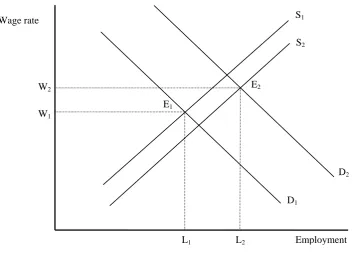
A shortage of a particular skill is said to exist when employers are unable to fill, or have considerable difficulty filling, vacancies for that skill at current levels of remuneration and conditions of employment, and reasonably accessible location. In terms of the simple demand and supply diagram for the skill shown in Figure 1, a shortage represented by (L2 –L1) exists when the wage rate W1 is below the equilibrium rate W0.

7

See Ageing Research Online (http://www.aro.gov.au/) and the links to related sites contained therein.

8

(12)

Skills shortages are to be distinguished from skills gaps and recruitment difficulties. Skills gaps occur when existing employees do not have the required qualifications, experience or specialised skills to meet a firm’s needs for an occupation. Recruitment difficulties occur when employers have some difficulty in filling vacancies for an occupation and may be due to factors such as relatively low remuneration, unsatisfactory working hours, an inaccessible location or ineffective recruitment procedures9.

When assessing the evidence for a skills shortage, the result depends on the aggregation, time and spatial dimensions under consideration. In general, the extent of the shortage increases with the level of disaggregation, decreases with the length of the time period, and decreases with the size of the geographical area10. Hence, while a skills shortage is conceptually well defined in terms of Figure 1, it is much more elusive to estimate empirically.

Figure 1. Excess Demand for Labour (Skills Shortage)

Skills shortages are usually measured by one of two methods - employer-based surveys or the analysis of labour market indicators. A recent example of the former is described in the World Class Skills for World Class Industries report prepared by the Allen Consulting Group

Wage rate

W0

W1

S

D E0

E2

E1

(13)

(2006). The quantitative information on skills shortages elicited by the survey is contained in Figure 4.3 of the report. It is reproduced here as Figure 2.

Note that no distinction is drawn between skills shortages and recruitment difficulties in the relevant survey question. Note also that the quantitative dimension is restricted to the percentage of respondents who reported difficulties in securing a particular skill, and does not extend to the amount by which the supply of the skill falls short of the demand for the skill. Most quantitative information from employer-based surveys takes this form.

Figure 2. Evidence of Skills Shortages from an Employer-Based Survey

64 48

46 36 36 35 26 19 15

0 10 20 30 40 50 60 70

Trades Technicians and paraprofessionals Engineering professionals Apprentices and trainees Managers Labourers and process workers Other professionals Clerical and administrators IT professionals

Pe r ce nt of s ample agre e ing

Source: Allen Consulting Group (2005). Difficulties securing skills—by occupation, Australian Companies, 2005. Survey question: In the last year has your company experienced difficulties in securing the following types of employees?

The market indicator approach does not attempt to measure skills shortages directly, but to infer their existence from changes in skilled vacancies, employment, unemployment, participation, hours worked and/or wages11. The most influential example of the method is the Skills in Demand program operated by the Department of Education, Employment, and Workplace Relations (2006) on an annual basis. It relies in part on the Survey of Employers who have Recently Advertised (SERA) and forms the basis of the Migration Occupations in Demand List (MODL) maintained by the Department of Immigration and Citizenship. It has the limited objective of providing qualitative, indicative information only on skills in demand.

10

For further discussion on this issue, see Shah and Burke (2006).

11

(14)

Returning to Figure 1, no direct information on the extent of skills shortages, as measured by the excess demand (L2 – L1), is published in Australia.

In a market economy, skill shortages are a transient phenomenon. Referring again to Figure 1, the existence of the excess demand (L2 – L1) will induce an increase in the wage rate and a movement along the supply curve from E1 to E0, thus eliminating the shortage. However, if the market mechanism is deemed to be too slow, policies which increase labour market flexibility may be appropriate. Alternatively, if the wage rate W0 is deemed to be too high, policies designed to shift the supply curve to the right (by additional training programs or increased immigration, for example) would restore equilibrium at a lower rate.

(15)

Figure 3. Shifts in Demand and Supply over Time

3. Specifying the Simulations

In this paper, population ageing is characterised by its effects on labour supply by skill, on private consumption by commodity, and on government consumption by commodity. The specification of each of these effects is discussed in turn.

3.1 Labour Supply

For the basecase simulation, labour supply was determined by progressively projecting the following variables:

• adult population,

• labour force participation rates,

• labour force measured in persons,

• unemployment rates,

• employment measured in persons,

• average hours worked,

• employment measured in hours.

Employment Wage rate

W2

W1

S1

D1

E2

E1

L1 L2

S2

(16)

All these projections were taken from the Productivity Commission’s report and are differentiated by age and sex.

A skill dimension was then incorporated into the projections using data from the Labour Force Survey (LFS) and the Survey of Education and Work (SEW), both of which are conducted by the Australian Bureau of Statistics (ABS) on a regular basis. Specifically, a five-dimensional employment matrix (measured in persons) was constructed for each year from 1994-95 to 2003-04, its dimensions consisting of

• qualification level (7 levels of highest educational attainment),

• qualification field (12 main fields of highest educational attainment),

• occupation (81 minor occupational groups),

• sex (2) and

• age (12 groups).

The qualification categories belong to the Australian Standard Classification of Education (ASCED) (ABS, 2001) and the occupations belong to the Australian Standard Classification of Occupations (ASCO) (ABS, 1997).

Next, two three-dimensional employment matrices (one measured in persons and one measured in hours) were constructed for each year, the dimensions being

• occupation (81 minor occupational groups),

• sex (2) and

• age (12 groups).

(17)

For the counterfactual simulation, the adult population was assumed to grow at the same rate as in the basecase but its distribution by age and sex remains as it was in 2003-04. The resulting employment growth rates by skill for the two simulations are compared in Table A1 of the Appendix. Population ageing has the effect of reducing the average annual rate of growth in employment from 1.00 per cent per annum in the counterfactual (no ageing) simulation to 0.81 per cent per annum in the basecase (ageing) simulation.

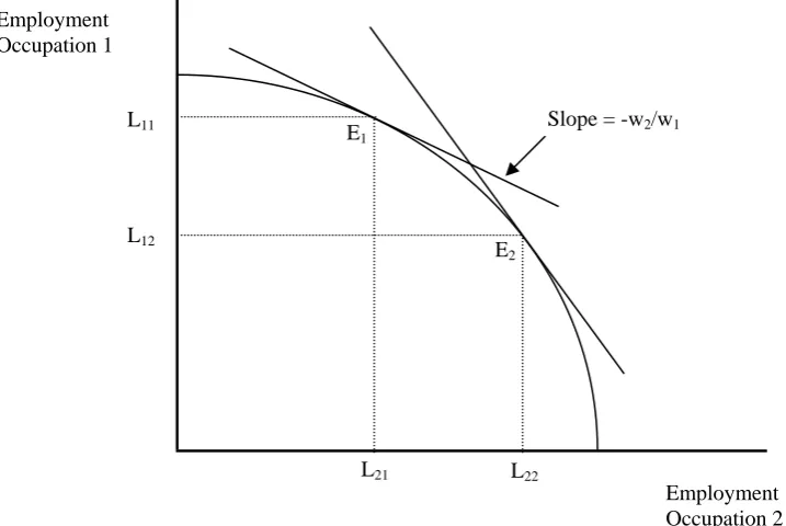
In order to support the simulations, the MONASH model was augmented with CET-like skill-specific occupational supply functions. For holders of a given skill, these functions make labour supply to individual occupations a positive function of the relative wages of those occupations12. Figure 4 presents the idea diagrammatically. The position of the transformation curve is determined by the employment level of the skill. If the wage rate of occupation 2 increases relative to that of occupation 1, the isorevenue line becomes steeper, and the owners of the skill can increase their income by transforming some of occupation 1 into occupation 2. Hence, they change the occupational mix from E1 to E2. In principle, each of the 64 skills can be transformed into any of the 81 occupations identified in the model. However, if none of a particular skill is used in a particular occupation in the base period, none of it will be used in that occupation in the simulations.

12

(18)

Figure 4. Skill Transformations between Occupations

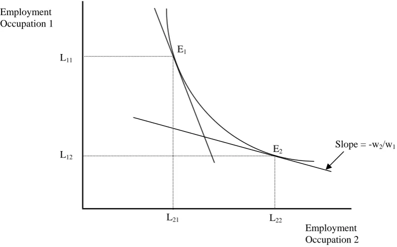
Labour of different occupations can be converted, in turn, into effective units of industry-specific labour according to Constant Elasticity Substitution (CES) functions. In Figure 5, the position of the isoquant is determined by the level of employment in the industry. If the wage rate of occupation 2 decreases relative to that of occupation 1, the isocost line becomes steeper, and the producers in the industry can reduce their costs by substituting some of occupation 2 for occupation 1. Hence they change the occupational mix from E1 to E2. In principle, each of the 106 industries can employ any of 81 occupations but, as before, none of a particular occupation will be used by an industry in the simulations if none of it was used by that industry in the base period.

According to this treatment, then, when Figure 3 refers to a skill (the employment of which is exogenous), the supply curves should be vertical. When it refers to an occupation (the employment of which responds to changes in wage rates), the supply curves should be upward sloping.

Employment Occupation 1

Slope = -w2/w1

E2

E1

L21 L22

Employment Occupation 2 L11

(19)

Figure 5. Substitution between Occupations in Industries

3.2 Private Consumption

The 2003-04 Household Expenditure Survey (HES) contains information for households (6975 records), for persons (13726 records) and for expenditure (492477 records) on 625 commodities. In principle, the direct effect of population ageing on household expenditure by commodity can be determined by:

(a) calculating per capita expenditure on each of the 625 commodities by age and sex in 2003-04;

(b) calculating the expenditures in the years 2004-05 to 2024-25 on the assumption that the population by age and sex grows as described in the Productivity Commission’s report, and that per capita expenditure by age and sex remains constant;

(c) calculating the expenditures in the years 2004-05 to 2024-25 on the assumption the total population grows as in step (b), and that both the distribution of the population by age and sex and per capita expenditure by age and sex remain constant;

(d) subtracting the expenditures calculated at step (c) from the expenditures calculated at step (b).

Employment Occupation 1

Slope = -w2/w1

E2

E1

L21 L22

Employment Occupation 2 L11

(20)

However, the expenditure records in the HES are household specific rather than person specific, and the age and sex of a household are not defined. Hence the following algorithm was designed.

(a) The HES describes how the 2003-04 population (population 1, say) by age and sex is distributed between 6957 households. In this distribution, each person has the same weight as the household weight.

(b) A new population (population 2, say) is calculated in which the number of persons is the same as population 1 but the distribution across age and sex is the same as the population projected by the Productivity Commission for 2004-05.

(c) Population 2 is distributed between the 6957 household types by adjusting the household weights. In this distribution, each household type has the same number of persons of a particular age and sex as in population 1, and each person has the same weight as the household weight.

(d) Steps (b) and (c) are repeated for populations 3 to 22 corresponding to the years 2005-06 to 2024-25.

(e) The expenditures on each of the 625 HES commodities is then calculated for each of the 22 populations on the assumption that both the expenditure per household and the distribution of expenditure between persons within a household remain constant. Differences between the expenditures of the populations are due entirely to differences in the numbers of households of each of the 6957 types.

(f) The direct effect of population ageing on expenditures between years 2004-05 and 2005-06, say, is then determined by subtracting the expenditures of population 2 from those of population 3.

The details of the algorithm are set out in Giesecke and Meagher (2008).

(21)

was allocated between the HES households in proportion to the estimated sale price of their dwellings, a category that is included in the HES data. In like manner, several of the expenditure categories included in the HES are not included in HFCE and were excluded from the data for the simulations. Finally the HES data was aggregated to a classification compatible with HFCE data, and scaled to conform to the latter for 2003-04.

The revised data were then aggregated across households using the 22 sets of household weights derived via the algorithm described above. The changes in the resulting expenditure shares then represent the direct effect of population ageing on household consumption.

3.3 Public Consumption

In its report, the Productivity Commission discusses the projected effects of population ageing on government expenditure for several categories, including health, education and aged care. The database for the MONASH model identifies Government Final Consumption Expenditure (as defined in the National Accounts) by input-output commodity. The commodity classification includes health and education, but they are not conceptually the same as the corresponding categories used by the Commission. The latter are much larger. Evidently, the Commission has included in its definition of government expenditure categories (such as transfer payments) which are not included in National Accounts definition. For example, aged care is a component of the commodity Community services in the National Accounts. However, the Commission’s estimate of expenditure on aged care significantly exceeds the National Accounts estimate of expenditure on all components of Community services. No attempt has been made to reconcile these differences quantitatively. Rather, it has been assumed

(a) that the effects of population ageing on the National Accounts’ versions of government expenditure on health and education are the same as the effects on the Commission’s versions, and

(22)

4. The Simulation Results

As previously indicated, the effects of population ageing are modelled by comparing two economies: a basecase in which population ageing takes place, and an alternative (counterfactual) economy in which the age structure of the population remains unchanged. In the interests of transparency, various components of the comparison are identified separately via separate simulations. In particular, the total effect of population ageing is decomposed into:

• a scale effect due to age-related shifts in total hours of employment (with the skill composition of employment unchanged).

• a skill effect due to age-related shifts in hours of employment distinguished by skill (with total hours of employment unchanged),

• a taste effect due to age-related shifts in the commodity composition of household final consumption, and

• a public effect due to age-related shifts in government final consumption,

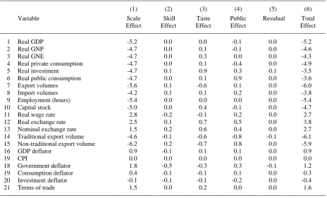
The simulations generate results for each year from 2004-05 to 2024-25. However, the discussion will concentrate on explaining the deviations in the levels of selected variables in the basecase (ageing) simulation from their values in the counterfactual (no ageing) simulation in the final year, i.e., 2024-25. These deviations are reported Tables A2 to A9 in the appendix. Each table contains six columns, the first four of which correspond to the scale, skill, taste and public effects just described. The model is non-linear, so the sum of the four component effects differs slightly from the total effect. The difference is reported as a residual in the fifth column. The final column contains the total effect and is the sum of the other five.

According to column 6, row 1 of Table A2, real GDP is 5.2 per cent smaller in the basecase than it is in the counterfactual . In what follows, it will often be said of this kind of result that population ageing “causes” real GDP to “decrease” by 5.2 per cent.

4.1 The Scale Effect

(23)

types of labour differentiated by skill (Tables A6 and A7, column 1) fall by the same amount. It is assumed that, in the counterfactual simulation, investors are aware of the prospects for decreased labour supply. Hence the deviation in the capital stock (Table A2, column 1, row 10) almost matches the deviation in employment (row 9). However the capital deviation is slightly smaller because the economy is smaller in the basecase simulation (row 1) and thus the deviation in the terms of trade is positive (row 21). With a smaller economy, the volume of imports required to sustain production (row 1) and meet consumption and investment demands (rows 4 to 6) is reduced. Lower import volumes (row 8) can be financed with lower export volumes (row 7). Foreign demands are modelled in MONASH via downward-sloping constant elasticity demand schedules. Hence, as export volumes contract, the foreign currency prices of exports rise. As foreign currency import prices are exogenous, this accounts for the improvement in the terms of trade. This improvement, together with the fall in the relative cost of capital (compare rows 16 and 20), accounts for the less rapid decline in capital relative to labour supply. With better terms of trade, a given volume of imports can be financed by a smaller volume of exports. Hence the real exchange rate appreciates (row 12) and the real balance of trade (rows 7 and 8) moves towards deficit.

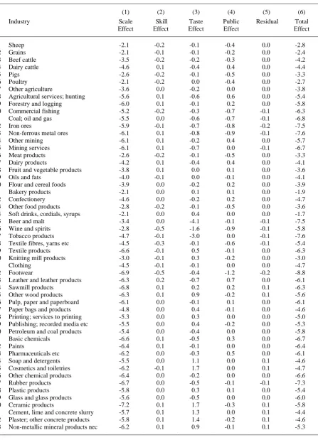
Table A3 presents output results for 106 industries. Consistent with the contraction in aggregate activity (row 1, Table A2) and its relatively uniform distribution between the expenditure-side components of GDP (rows 4 to 8), all industrial sectors contract. From the preceding discussion of macro results, the contraction in aggregate employment causes the real exchange rate to appreciate. In general, this has a negative effect on the output of industries producing export and import-competing commodities, and explains the unfavourable output rankings of such trade-exposed industries as Footwear (row 32, Table A3) and Motor vehicles and parts (row 59). With real consumption decreasing (row 4, Table A2) but population unchanged, per-capita income decreases. This restricts demand for the income-elastic commodity Ownership of dwellings (row 92, Table A3). As the size of the housing stock falls, output of sectors involved in dwellings construction also contract, leading to the relatively weak output performance of industries such as Sawmill products (row 34, Table A3), Ceramic products (row 50) and Residential building (row 75).

(24)

output deviation of only 2.1 per cent, well below the 5.5 per cent for output as a whole (row 1, Table A2). Sheep, Grains, Beef cattle, Dairy cattle, Pigs and Other agriculture all use agricultural land (in addition to labour and capital) as a primary factor input. In the basecase simulation, aggregate activity decreases, causing the demand for agricultural commodities to contract. However, the supply of agricultural land is held at the same level as in the counterfactual, and agricultural industries have only a limited ability to substitute between land and other primary factors. Hence the rental rate on agricultural land decreases and feeds into the prices of agricultural goods. This is apparent in column 1 of Table A4, which shows that agricultural industries experience relatively large decreases in per-unit production costs. This has a number of implications for activity in agricultural and related industries. Firstly, these industries export a relatively high proportion of their output, and export demand elasticities are high compared to domestic price elasticities. As a result, agricultural industries experience positive deviations in export volumes. This explains why the decrease in the volume of traditional export (which includes agricultural exports) is less than the decrease in aggregate exports (compare rows 7 and 14, Table A2). Agricultural commodities are also important inputs into domestic agricultural processing industries. Hence the decrease in agricultural commodity prices causes a decrease in costs for domestic agricultural processing industries. This can be seen in Table A4, which shows that industries such as Meat products (row 16), Dairy products (row 17), Fruit and vegetable products (row 18), Other food products (row 23), and Wine and spirits (row 26) experience comparatively large decreases in costs. The products produced by agricultural processing industries also tend to have relatively low income elasticities, and hence they are not affected to the same degree as other industries by the 4.7 per cent fall in real consumption spending (Table A2, row 4). This accounts for the high output ranking (or relatively small reduction in output) of industries such as Bakery products (row 21), Poultry (row 6), Soft drinks, cordials and syrups (row 24), Beer and malt (row 25), Flour and cereal foods (row 20), and Oils and fats (row 19).

(25)

fixed supply of land in the agriculture sector, where these occupations are mostly employed. For agricultural industries to contract, they must substitute away from labour (and capital) to the detriment of employment of the occupations used intensively in agriculture. Other occupations experiencing above average employment decreases are tradespersons, engineers and labourers. These occupations are used in mining and construction, industries which experience above average output deviations. Among the occupations experiencing below average employment deviations are Shop managers (row 28), Food tradespersons (row 43), Sales assistants (row 72), Elementary food preparation workers (row 80), and Hospitality workers (row 62). These occupations are employed predominantly in the food processing industries and the retail trade and hospitality industries. As discussed earlier, food processing industries experience low output deviations because of input cost reductions, and because the markets for their products that are simultaneously price-elastic and income-inelastic. This leads to low output deviations for the retail trade and hospitality industries, as the margin services they provide are important in facilitating the sale of commodities produced by food processing industries.

4.2. The Skill Effect

The second column of Tables A2 to A9 identifies the impact of age-related changes in the skill composition of the workforce, holding employment, household tastes, and government spending at their counterfactual levels. It is clear from Table A2 that the skill effect alone has little impact on the macroeconomy. This largely follows from the assumption that the skill effect does not result in any age-related deviation in total hours of employment (row 9). It also follows that, for different kinds of labour, the skill effect will cause employment to rise for some and fall for others.

(26)

Table A7 reports the employment deviations for cross-classified qualification levels and fields. These deviations are exogenous to the simulations, their derivation having been described previously in Section 3. The ranking of the employment deviation for a particular occupation (see Table A5) is largely determined by the employment deviations of the skills that are used intensively in that occupation. For example, Building and engineering associate professionals (row 25), Mechanical engineering tradespersons (row 36), Fabrication engineering tradespersons (row 37), Automotive tradespersons (row 38), Electrical and electronics tradespersons (row 39), Printing tradespersons (row 46) and Wood tradespersons (row 47) are among the occupations experiencing the largest positive employment deviations in column 2 of Table A5. All these occupations are important employers of persons with engineering skills and, from Table A7, most of those skills experience relatively large positive employment deviations (see rows 3, 12, 34, 45, and 56 of column 2). A similar story underlies the favourable occupational employment outcomes for School teachers and Enrolled nurses (rows 17 and 31, respectively, of Table A5). From Table A7, the skill effect results in positive employment deviations for all education qualifications (see rows 7, 17, 27, 38 and 48) and many holders of these skills are employed as School teachers. The employment outcome for Enrolled nurses follows from the positive employment deviations for Health qualifications at the Diploma level (Table A7, row 37) and the Certificate III and IV level (row 49).

Among the occupations experiencing the largest negative employment deviations, Food tradespersons (Table A5, row43) and Hairdressers (row 48) owe their ranking to the large deviation for the skill Food, hospitality and personal services, Certificate III and IV (Table A7, row 53). Most Management qualifications experience negative employment deviations (see Table A7, rows 18, 28, 39, and 50), and this contributes to the low employment ranking for occupations such as Accountants (Table A5, row 10), Computing professionals (row 12), Finance associate professionals (row 26), and Intermediate numerical clerks (row 57). The result for Computing professionals is enhanced by the negative employment deviation for skill Information technology, bachelor degree (Table A7, row 22)).

(27)

rise in occupations that use engineering skills intensively. This is achieved via a negative deviation in the wages of occupations that typically require engineering skills. The mechanism is also useful for understanding the industry cost results in Table A4. The largest per-unit cost decreases, relative to the counterfactual, are experienced by Railway equipment (row 61), Aircraft (row 62), Other machinery and equipment (row 68), Mechanical repairs (row 79), Other repairs (row 80), Education (row 99), and Health services (row 100). Cost decreases for these industries are due to negative wage deviations for occupations such as teachers, tradespersons, and nurses. As discussed earlier, these occupational wage reductions can be traced back to positive deviations in the supply of skills relating to engineering, education and health.

Some of the largest positive deviations in per-unit costs are experienced by Retail trade (Table A4, row 78), Accommodation cafes, restaurants (row 81), Banking (row 88), Non-bank finance (row 89), Insurance (row 90), Services to finance (row 91), Legal and accounting services (row 95), Libraries and museums (row 103) and Personal services (row 105). Generally, this is due to the positive wage deviations experienced by occupations such as Accountants (Table A5, row 10), Computing professionals (row 12), Finance associate professionals (row 26), Food tradespersons (row 43), Hairdressers (row 48), and Hospitality workers (row 62). In turn, these positive occupational wage outcomes can be traced back to negative deviations in employment of workers with skills in Management and Food, hospitality and personal services. An exception is Libraries and museums, which experiences a positive cost deviation because of a negative deviation in the supply of workers with a Bachelor degree or a Diploma in the Creative arts (Table A7, rows 30 and 41, respectively)

4.3. The Taste Effect

(28)

The ten commodities experiencing the largest (weighted by budget share) age-related downward shifts in household consumption due to ageing are, in order of biggest shift to smallest shift: Education, Motor vehicles and parts, Accommodation cafes and restaurants, Tobacco products, Retail trade, Beer and malt, Petroleum and coal products, Wine and spirits, Banking, and Electronic equipment. Hence, in comparing the basecase (ageing) scenario against the counterfactual (no ageing) scenario, the industries producing these commodities are among those experiencing the largest negative output deviations (see Table A3). On the other hand, the ten commodities experiencing the largest upward shifts are, in order of biggest shift to smallest shift: Ownership of dwellings, Insurance, Cosmetics and toiletries, Communication services, Personal services, Other services, Publishing and

recorded media, Water sewerage and drainage services, and Electricity supply. Hence, the industries producing these commodities are among those experiencing the largest positive output deviations when the basecase is compared to the counterfactual.13

The implications of the taste effect for the macroeconomy are small (Table A2). Broadly speaking, the taste effect shifts demand in favour of capital-intensive commodities, reflecting the top ranking of Ownership of dwellings among those commodities experiencing positive preference shifts due to ageing. As a result the capital stock and, concomitantly, real investment both rise slightly relative to the counterfactual (see rows 10 and 5, respectively). Since labour supply (row 9) is not affected by the taste effect, there is no discernible change in real GDP (row 1). The positive deviation in real investment then implies a rise in real GNE relative to GDP, and the balance of trade moves towards deficit. This outcome is facilitated by a real appreciation (row 12), leading to a negative deviation in export volumes (row 7) and a positive deviation in import volumes (row 8). The negative deviation in exports causes a small positive deviation in the terms of trade (row 23) and an associated small increase in real GNP (row 2). The macro closure requires real private and public consumption spending to move with real GNP. Hence, with real GNP higher than counterfactual, so too are private and public consumption spending (rows 4 and 6, respectively).

13

(29)

Real appreciation has a negative impact on trade-exposed industries. This accounts for the negative output deviations of the agricultural and mining industries (rows 1 to 15, Table A3), and import-competing industries such as Clothing (row 31), Footwear (row 32) and Motor vehicles and parts (row 59).

Turning to occupational employment (Table A5), the largest negative deviations are recorded by occupations related to education, namely, University and vocational education teachers (row 18), Miscellaneous education professionals (row 19) and School teachers (row 17). Other large deviations are recorded by Hospitality workers (row 62) and Hospitality and accommodation managers (row 29), occupations for which employment is concentrated in the Accommodation cafes and restaurants and Retail trade industries. Both these industries suffer adverse age-related shifts in household preferences due to ageing. Since these adverse age-related preference shifts are excluded from the counterfactual simulation, these industries do comparatively poorly when the basecase simulation is compared with the counterfactual simulation. Farm managers (row 7), Skilled agricultural workers (row 44) and Agricultural and horticultural labourers (row 79) experience small negative deviations because export-oriented agricultural industries suffer from the real appreciation. Similarly, employment of Automotive tradespersons (row 38) and Mechanical engineering tradespersons (row 36) suffer from the appreciation via its effect on the import-competing Motor vehicles and parts industry. Finally, the occupation Carers and aides (row 61) is adversely affected by the taste effect because the industry Education accounts for just over twenty per cent of its employment.

(30)

inclusion of age-related shifts in preferences towards Communication services (Table A3, row 87).

4.4 The Public Effect

According to the method described in Section 3.3, relative to counterfactual, population ageing will result in an increase in public spending on health of about 16 per cent by 2024-25, a decrease in education spending of about 17 per cent, and an increase in spending on aged care of about 50 per cent. The impacts on industry outputs of including these age-related changes are shown in Table A3. For Education (row 99), output decreases by 5.5 per cent relative to the counterfactual, while it increases by 5.4 per cent for Health services (row 100) and by 15.9 per cent for Community services (row 101).

In modelling the public effect, the 106 commodities identified in MONASH are divided into two sets: those which are likely to be directly affected by population ageing, and those which are not. The former set consists of education, health, and community services. The latter consists of all other commodities. A stylised14 representation of the treatment of percentage changes in public demand for commodity i (xgovi) in each year is given by equations of the form:

xgovi = realcons + fxgovi ,

where realcons is the percentage change in real private consumption spending, and fxgovi is an exogenous shift term. In columns (4) and (6) of Tables A2 to A9, age-related changes in public consumption are implemented by shocking fxgovhealth, fxgoveducation, and

fxgovcommunity_services. In all other columns, aggregate public consumption moves with aggregate private consumption (see Table A2, rows 4 and 6), and the commodity-composition of public consumption is unchanged. This explains why, in column (4), the output of Government administration (Table A3, row97) and Defence (row 98) decrease by 0.1 per cent relative to the counterfactual.

14

(31)

Changes in the commodity-composition of public spending have little effect on the economy’s stocks of capital and labour, and hence have little effect on real GDP and real GNP (Table A2, rows 1 and 2, respectively). Aggregate (private plus public) real consumption spending is assumed to move with real GNP in all the simulations. Hence, the public effect of population ageing leaves aggregate consumption spending largely unchanged. However the net effect of: (a) including age-related shifts in public consumption and (b) indexing the remaining elements of public consumption to private consumption, is to increase public consumption spending by 0.9 per cent (Table A2, row 6). This increase in public consumption requires private consumption to fall by 0.4 per cent relative to the counterfactual.

(32)

wage increases of around 15 per cent relative to counterfactual. In practice, the upward pressure on wages in health-related occupations can be expected to induce changes that are not modelled in the present simulations, such as increased enrolments in courses leading to the acquisition of medical skills, and increased intakes of immigrants with medical skills. For this reason, the wage outcomes should not be interpreted as projections but as indicators of adjustment pressure. The simulation suggests that population ageing generates a need to ensure that education and training policy settings facilitate the flexible flow of training resources towards the provision of health-related skills, in order to offset age-related cost pressures.

5. Implications for public policy

(33)

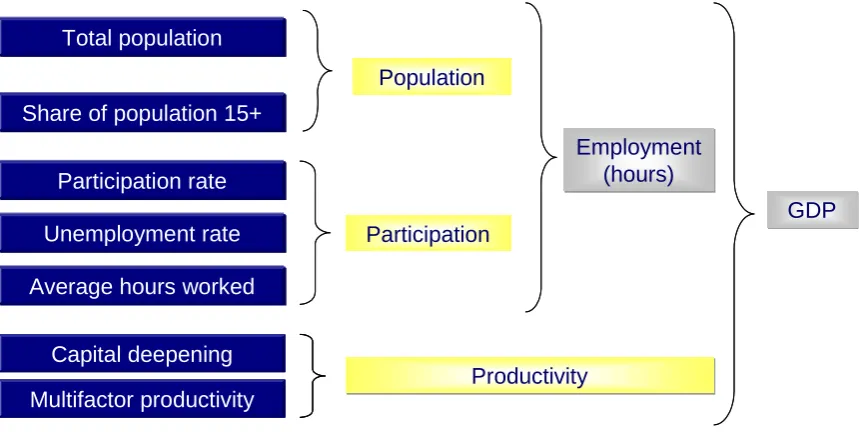
Figure 6. Economic Growth and the Three 'Ps'

Growth prospects

Components of GDP

Participation Participation Population Population

Employment (hours) Employment

(hours)

GDP GDP Total population

Share of population 15+

Participation rate

Unemployment rate

Average hours worked

Productivity Capital deepening

Multifactor productivity Capital deepening

Multifactor productivity Multifactor productivity

Source: Henry (2002).

All three reports paid particular attention to the commodity composition of government expenditure in so far as it affects education, health and aged care. However, their primary concern was with macroeconomic issues and those issues have largely driven the policy debate. The contribution of the present study is to add some structural “flesh” to those macro “bones”, and hence to provide the wherewithall for a more discursive policy discussion. In so doing, the study has canvassed effects arising from the interaction between demand and supply in the markets for different types of labour and for commodities. This is an advance over the analyses in the aforementioned reports which treat labour supply and (selected) commodity demands as evolving independently of each other.

(34)

likely that workers will respond to the improving remuneration of skills in health relative to skills in education long before 2024-25 is reached. The results for wage rates should thus be interpreted as a guide to training and education policy makers, marking likely areas of future training demand pressures. In future work, it is planned to use the model to solve for the changes in skill supply required to maintain targetted wage relativities.

Clearly, the simulations do not provide unconditional labour market forecasts. On the other hand, they do reveal the kind of structural pressures which are implicit in fiscal gap analyses like those conducted by the Treasury (in its Intergenerational Reports) and the Productivity Commission (in its Economic Implications Report). In those analyses, demand and supply are projected independently of each other and any structural tension between the two goes unobserved. According to the present simulations, the fiscal gap projections rely, inter alia, on a change in the mix of skilled labour away from education towards health, be it by government policy intervention or by the operation of market forces. In the absence of such a change in employment, relative wage rates will adjust instead, disrupting the projections of government spending and hence the projections of the fiscal gap. An important function of the simulations, then, is to complement the earlier studies by drawing out the structural implications that underlie their projections.

The foregoing considerations are also relevant to gap analysis when it is applied to labour markets15 rather than government budgets. In that case, the supply of labour by skill and/or occupation is projected independently of demand, and demand is projected on the assumption that relative wage rates remain constant. It follows that the economy can only “adjust” to developing labour market pressures by increases in unemployment (surpluses) or by increases in the excess demand for labour (shortfalls). Surpluses and shortfalls are then taken to represent the amounts by which the government should adjust the training regime embodied in the supply projections. Thus a shortfall is interpreted to be a projection of the skills shortage that will arise if the government does not change its policy. However, in a market economy, relative wage rates will respond to demand pressures and labour supply will respond to changes in relative wage rates. Hence the projected shortages will fail to

15

(35)

materialise regardless of whether the government adjusts its policy. As a method for projecting future skill shortages, gap analysis has little credibility16.

The result with respect to health and education, while striking, is not surprising and has been widely anticipated in other studies. A related result which has not received so much attention is the relatively small size of the taste effect relative to the public effect, especially as they relate to health and education. The main reason is simply that the public sector dominates expenditure on these two commodities. However, public expenditure is also more age-sensitive than private sector expenditure. Health costs are predominantly incurred in the last years of life and the government expenditure is concentrated on those years to a greater extent than private sector expenditure. While the taste effect is generally less important than the public effect, the position is reversed for some occupations. As the population ages, private consumption shifts towards personal services and ownership of dwellings. Hence hairdressers and workers in some construction-related occupations experience significant positive deviations in their wage rates due to the taste effect. This example illustrates the capacity of the decomposition methodology to expose the diverse effects of population ageing on the structure of the economy, effects that would otherwise be exceedingly difficult to anticipate.

The key role of education and health suggests that the emphasis in the earlier Treasury and Productivity Commission studies was not misplaced. On the other hand, some of the other structural results are quite significant for aspects of the current policy debate. Firstly, for skilled labour, population ageing tends to create pressure on the supply with qualifications in the trades rather than in higher education. As before, this pressure is evidenced by the wage rate deviations reported in Table A9. Thus population ageing tends to offset the requirements for more university, rather than TAFE, training places that some commentators perceive to flow from the present round of skill shortages17. Furthermore, the pressure (or lack thereof) is not uniform, with the skill level Graduate diploma or certificate particularly tending towards oversupply. Even more interesting is the tendency of population ageing to create excess demand for persons with No post-school qualification. This result sits uneasily with the almost universal policy emphasis on the need for a more highly skilled workforce. It does, however, lend some collateral relevance to the position adopted by Saunders (2007, 2008),

16

(36)

who argues that more education and training is not the answer to skills shortages because of the limited ability of unskilled workers to benefit from such training.

Finally, it is important to note the wide range of the deviations in the occupational wage rates reported in Table A8. Most of the outliers can be obviously attributed to education and health, and hence tend to be exaggerated because of the limited avenues for adjustment allowed in the simulations. However, even within an occupational group like Tradespersons (rows 35 to 50), there is considerable variation. In other words, the simulations indicate that it is not safe to generalise about the effects of population ageing on the labour requirements for an ostensibly homogeneous occupation like tradespersons, let alone much more diverse groups like Persons with a trade qualification or Skilled labour as a whole18. Evidently, labour market policies predicated on ideas formed at high levels of aggregation are unlikely to apply satisfactorily at lower levels of aggregation.

6. Concluding Remarks

This paper has presented an analysis of the likely effects of population ageing on the structure of the Australian economy during the period from 2004-05 to 2024-25. The analysis is based on simulations using a suitably modified version of the MONASH applied general equilibrium model. It is comprehensive in that it is conducted on an economy-wide basis. It is very detailed in that it encompasses 64 skill groups, 81 occupations and 106 industries. It is coherent in that every part of the analysis is consistent with every other part.

The analysis is not without its limitations. In common with every other forward-looking analysis, its results are subject to uncertainty. Moreover, the level of uncertainty increases with the level of detail and with the length of the time horizon. This circumstance has sometimes lead to the belief that, for policy purposes, formal labour market analysis should be restricted to high levels of aggregation and/or short time horizons19. In the case of population ageing at least, the analysis presented here strongly suggests that such a strategy is unlikely to produce good policy outcomes. The effects within more highly aggregated categories are

17

See Birrell and Rapson (2006) and Birrell, Healy and Smith (2008).

18

(37)

simply too diverse. In any case, formal techniques allow large amounts of relevant data to be brought to bear in a consistent manner, and that advantage that should not be lightly forgone.

A formal model-based economic analysis, like all other economic analyses, is also limited by the quality of the theory and data on which the analysis is based. In the present case, care had to be taken in interpreting the wage rate results because of the restricted treatment of the markets for labour of different skills. That limitation could be alleviated in the future by the introduction of additional economic theory. In the meantime, its implications for policy formulation could be assessed by means of sensitivity analysis. As the theory and data incorporated in an analysis can almost always be improved, the capacity for interim sensitivity analysis is a considerable advantage of formal analysis. Furthermore, such analyses can be used to assess quantitatively the relative merits of different policy options under consideration. In other words, simulations of the kind presented here can contribute to an understanding of the implications, not only of population ageing itself, but also of the policy responses designed to ameliorate its effects.

Finally, formal analyses can be readily revised as economic circumstances change. The specification of the simulations determines the environment in which population ageing is assumed to occur. For policy purposes, the usefulness of the analysis would be reduced if, say, the economy were to suffer a severe recession in the next few years. However, the usefulness of the methodology would remain undiminished as the simulations could simply be repeated with a more appropriate specification. In a recent presentation on population ageing, the Chairman of the Productivity Commission proffered the opinion that

“..even with all the uncertainties, there are good reasons for intelligent prognostication, provided that projections are updated as new information becomes available.” (Banks, 2004, p.26)

(38)

References

Access Economics (2005), Improved Forecasts of Employment Growth and Net Replacement Rates, report prepared for the Victorian Office of Training and Tertiary Education,

January.

Australian Bureau of Statistics (1997), ASCO - Australian Standard Classification of Occupations, Second Edition, Catalogue No. 1220.0.

Australian Bureau of Statistics (2000), Australian System of National Accounts: Concepts, Sources and Methods, Catalogue No. 5216.0.

Australian Bureau of Statistics (2001), Australian Standard Classification of Education (ASCED), Catalogue No. 1272.0.

Australian Bureau of Statistics (2005), “Skills Shortages in Western Australia”, Western Australian Statistical Indicators, Catalogue No. 1367.5, December Quarter.

Australian Bureau of Statistics (2006), Household Expenditure Survey and Survey of Income and Housing – Confidentialised Unit Record Files, Technical Paper, Australia, 2003-04, Catalogue No. 6540.00.001.

Australian Bureau of Statistics (2007), Australian System of National Accounts, 2006-07, Catalogue No. 5204.0.

Australian Treasury (2002), Intergenerational Report 2002-03, Canberra. Australian Treasury (2007), Intergenerational Report 2007, Canberra.

Allen Consulting Group (2005), World Class Skills for World Class Industries: Employers’ Perspectives on Skilling in Australia, Report to the Australian Industry Group, Melbourne. Banks, G. (2004), “An Ageing Australia: Small Beer or Big Bucks?”, presentation to the

South Australian Centre of Economic Studies, Adelaide, April.

Birrell, B. and V.Rapson (2006), “Clearing Away the Myths: Higher Education’s Place in Meeting Workforce Demands”, paper prepared for the Dusseldorp Skills Forum, October. Birrell, B., E.Healy and T.F.Smith (2008), “Labor’s Education and Training Strategy:

Building on False Assumptions?”, People and Place, 16 (1), 40-54.

Department of Employment and Workplace Relations (2005), Workforce Tomorrow: adapting to a more diverse Australian labour market, Canberra.

(39)

Dixon, P.B. and M.T.Rimmer (2002), Dynamic General Equilibrium Modelling for Forecasting and Policy: a Practical Guide and Documentation of MONASH, North-Holland, Amsterdam.

Dixon, P.B. and M.T. Rimmer (2006), “The Displacement Effect of Labour-Market Programs: MONASH Analysis”, Economic Record, 82 (special issue), S26-S40.

Downes,P. and A.Stoeclel (2007), “Drivers of structural change in the Australian economy”, Centre for International Economics, Canberra. Available from

http://www.thecie.com.au/publication.asp?pID=121 .

G.A.Meagher (2008), “Modelling the Economic Effects of Populating Ageing”, Working Paper No. G-172, Centre of Policy Studies, Monash University. Available from http://www.monash.edu.au/policy/elecpapr/g-172.htm .

Henry, K. (2002), “The Demographic Challenge to Our Economic Potential”, Chris Higgins Memorial Lecture, Canberra, November.

Independent Pricing and Regulatory Tribunal of New South Wales (2006), Upskilling NSW: How Vocational Education and Training Can Help Overcome Skill Shortages, Improve

Labour Market Outcomes and Raise Economic Growth, Sydney, December.

Leigh, A. (2008), “The Economics of Labour Shortages”, presentation at the Melbourne Institute Public Economics Forum on Boosting the Labour Supply, Hyatt Hotel, Canberra, 29 April.

Meagher, G.A. (2007), “Assessing the Reliability of the MONASH Labour Market Forecasts: Some Comments on a Report by the National Institute of Labour Studies, National Centre for Vocational Education Research, Adelaide, July.

Richardson, S. (2007), “What is a Skills Shortage”, National Centre for Vocational Education Research, Adelaide, February.

Richardson, S. and Yan Tan (2007), “Forecasting Future Skill Demands: What We Can and Cannot Know”, National Centre for Vocational Education Research, Adelaide, July. Saunders, P. (2007), “What Are Low Ability Workers To Do When Unskilled Jobs

Disappear? Part 1: Why More Education and Training Isn’t the Answer”, Issue Analysis No. 91, Institute for Independent Studies, December.

Saunders, P. (2008), “What Are Low Ability Workers To Do When Unskilled Jobs

Disappear? Part 2: Expanding Low-skilled Employment”, Issue Analysis No. 93, Institute for Independent Studies, February.

(40)

Shah, C. and G.Burke (2006), Qualifications and the Future Labour Market in Australia, report prepared for the National Training Reform Taskforce, November.

Shah, C., L.Cooper and G.Burke (2007), Industry Demand for Higher Education Graduates in Victoria in 2008 to 2022, report prepared for the Victorian Office of Training and Tertiary Education, October.

(41)

APPENDIX

(42)

Table A1. Employment Growth Rates, 2004-05 to 2024-25, Hours, Per Cent Per Annum

ASCED Levels of ASCED Broad Fields of Study Simulation Educational Attainment

Basecase Counter-factual

Post-graduate degree Natural and physical sciences 1.99 1.88

Information technology 1.87 2.08

Engineering and related technologies 1.78 1.75 Architecture and building 2.27 2.24 Agriculture and environmental studies 1.47 1.71

Health 1.78 1.71

Education 2.37 2.35

Management and commerce 2.07 2.10 Society and culture 1.75 1.82

Creative arts 1.92 1.86

Food, hospitality, personal services 0.00 0.00 Graduate diploma or certificate Natural and physical sciences 2.14 2.23

Health 2.08 2.20

Education 1.46 1.43

Food, hospitality, personal services 0.00 0.00 Bachelor degree Natural and physical sciences 1.46 1.54

Health 1.06 1.23

Education 2.06 2.07

Food, hospitality, personal services 1.91 2.09 Advanced diploma or diploma Natural and physical sciences 1.61 1.65

Health 1.18 1.19

Education 1.25 0.98

Food, hospitality, personal services 2.30 2.40

(43)

Table A1. (continued). Employment Growth Rates, 2004-05 to 2024-25, Hours, Per Cent Per Annum

ASCED Levels of ASCED Broad Fields of Study Simulation Educational Attainment

Basecase Counter-factual

Certificate III or IV Natural and physical sciences 2.38 2.37 Information technology 1.94 2.21 Engineering and related technologies 0.56 0.56 Architecture and building 0.50 0.67 Agriculture and environmental studies 2.04 2.10

Health 2.21 2.20

Education 2.12 2.14

Management and commerce 2.00 2.17 Society and culture 2.41 2.47 Creative arts 1.96 2.10 Food, hospitality, personal services 1.47 1.69 Certificate I or II Natural and physical sciences 4.67 4.57 Information technology 2.30 2.59 Engineering and related technologies 1.48 1.35 Architecture and building 2.07 2.49 Agriculture and environmental studies 1.57 1.68

Health 2.94 2.85

Education 0.00 0.00

Management and commerce 1.78 1.68 Society and culture 3.24 2.89 Creative arts 3.44 3.63 Food, hospitality, personal services 2.50 2.36 No post-school qualification 0.01 0.33

(44)

Table A2. Macroeconomic Variables, Percentage Deviations of Basecase from Counterfactual, 2024-25

(1) (2) (3) (4) (5) (6)

Variable Scale

Effect

Skill Effect

Taste Effect

Public Effect

Residual Total Effect

1 Real GDP -5.2 0.0 0.0 -0.1 0.0 -5.2

2 Real GNP -4.7 0.0 0.1 -0.1 0.0 -4.6

3 Real GNE -4.7 0.0 0.3 0.0 0.0 -4.3

4 Real private consumption -4.7 0.0 0.1 -0.4 0.0 -4.9

5 Real investment -4.7 0.1 0.9 0.3 0.1 -3.5

6 Real public consumption -4.7 0.0 0.1 0.9 0.0 -3.6

7 Export volumes -5.6 0.1 -0.6 0.1 0.0 -6.0

8 Import volumes -4.2 0.1 0.1 0.2 0.0 -3.8

9 Employment (hours) -5.4 0.0 0.0 0.0 0.0 -5.4

10 Capital stock -5.0 0.0 0.4 -0.1 0.0 -4.7

11 Real wage rate 2.8 -0.2 -0.1 0.2 0.0 2.7

12 Real exchange rate 2.5 0.1 0.7 0.5 0.0 3.8

13 Nominal exchange rate 1.5 0.2 0.6 0.4 0.0 2.7

14 Traditional export volume -4.6 -0.1 -0.6 -0.8 -0.1 -6.1

15 Non-traditional export volume -6.2 0.2 -0.7 0.8 0.0 -5.9

16 GDP deflator 0.9 -0.1 0.1 0.1 0.0 0.9

19 CPI 0.0 0.0 0.0 0.0 0.0 0.0

18 Government deflator 1.8 -0.5 -0.3 0.3 -0.1 1.2

19 Consumption deflator 0.4 -0.1 -0.1 0.1 0.0 0.3

20 Investment deflator -0.1 -0.1 -0.1 -0.2 0.0 -0.4

(45)

Table A3. Industry Outputs, Percentage Deviations of Basecase from Counterfactual, 2024-25

(1) (2) (3) (4) (5) (6)

Industry Scale

Effect Skill Effect Taste Effect Public Effect

Residual Total Effect

1 Sheep -2.1 -0.2 -0.1 -0.4 0.0 -2.8

2 Grains -2.1 -0.1 -0.1 -0.2 0.0 -2.4

3 Beef cattle -3.5 -0.2 -0.2 -0.3 0.0 -4.2

4 Dairy cattle -4.6 0.1 -0.4 0.4 0.0 -4.4

5 Pigs -2.6 -0.2 -0.1 -0.5 0.0 -3.3

6 Poultry -2.1 -0.2 0.0 -0.4 0.0 -2.7

7 Other agriculture -3.6 0.0 -0.2 0.0 0.0 -3.8

8 Agricultural services; hunting -5.6 0.1 -0.6 0.6 0.0 -5.4

9 Forestry and logging -6.0 0.1 -0.1 0.2 0.0 -5.8

10 Commercial fishing -5.2 -0.2 -0.3 -0.7 -0.1 -6.3

11 Coal; oil and gas -5.5 0.0 -0.6 -0.7 -0.1 -6.8

12 Iron ores -5.9 -0.1 -0.7 -0.8 -0.2 -7.5

13 Non-ferrous metal ores -6.1 0.1 -0.8 -0.9 -0.1 -7.6

14 Other mining -6.1 0.1 -0.2 0.4 0.0 -5.7

15 Mining services -6.1 0.1 -0.7 0.0 -0.1 -6.7

16 Meat products -2.6 -0.2 -0.1 -0.5 0.0 -3.3

17 Dairy products -4.2 0.1 -0.4 0.4 0.0 -4.1

18 Fruit and vegetable products -3.8 0.1 0.0 0.1 0.0 -3.6

19 Oils and fats -4.0 -0.1 0.0 -0.1 0.0 -4.1

20 Flour and cereal foods -3.9 0.0 -0.2 0.2 0.0 -3.9

21 Bakery products -2.1 0.0 0.1 0.1 0.0 -1.9

22 Confectionery -4.6 0.0 -0.2 0.2 0.0 -4.7

23 Other food products -2.8 -0.2 -0.1 -0.5 0.0 -3.6

24 Soft drinks, cordials, syrups -2.1 0.0 0.4 0.0 0.0 -1.7

25 Beer and malt -3.4 0.0 -4.1 -0.1 -0.1 -7.5

26 Wine and spirits -2.8 -0.5 -1.6 -0.9 -0.1 -5.8

27 Tobacco products -4.7 -0.1 -3.0 0.0 -0.1 -7.6

28 Textile fibres, yarns etc -4.5 -0.3 -0.1 -0.6 -0.1 -5.4

29 Textile products -6.6 -0.1 0.5 -0.1 0.0 -6.3

30 Knitting mill products -3.0 -0.1 0.3 -0.2 0.0 -3.0

31 Clothing -4.5 -0.1 -0.1 0.0 0.0 -4.7

32 Footwear -6.9 -0.5 -0.4 -1.2 -0.2 -8.8

33 Leather and leather products -6.3 0.2 -0.7 0.7 0.0 -6.1

34 Sawmill products -6.8 0.1 0.2 0.2 0.1 -6.3

35 Other wood products -6.3 0.1 0.9 -0.2 0.1 -5.6

36 Pulp, paper and paperboard -6.1 0.0 -0.1 0.1 0.0 -6.1

37 Paper bags and products -4.8 0.0 0.4 -0.1 0.0 -4.6

38 Printing; services to printing -5.3 0.0 0.3 0.0 0.0 -5.0

39 Publishing; recorded media etc -5.5 0.0 0.4 -0.2 0.0 -5.3

40 Petroleum and coal products -5.4 0.0 -0.4 0.0 0.0 -5.8

41 Basic chemicals -6.6 0.1 -0.5 0.3 0.0 -6.7

42 Paints -6.4 0.1 -0.1 0.0 0.0 -6.4

43 Pharmaceuticals etc -6.2 0.0 -0.3 0.5 0.0 -6.1

44 Soap and detergents -5.5 0.0 1.1 0.0 0.1 -4.6

45 Cosmetics and toiletries -6.2 -0.1 1.7 0.0 0.1 -4.7

46 Other chemical products -6.4 0.0 -0.2 0.0 0.0 -6.6

47 Rubber products -6.7 0.0 -0.5 -0.1 -0.1 -7.3

48 Plastic products -5.8 0.0 0.3 0.1 0.0 -5.4

49 Glass and glass products -5.6 0.0 -0.5 0.0 0.0 -6.0

50 Ceramic products -7.2 0.1 1.7 -0.3 0.1 -5.8

51 Cement, lime and concrete slurry -5.7 0.1 1.3 0.0 0.1 -4.4

52 Plaster; other concrete products -5.8 0.1 1.4 -0.2 0.1 -4.6

53 Non-metallic mineral products nec -6.2 0.1 0.9 -0.1 0.1 -5.3