Two dimensional angular domain optical imaging in biological tissues

(1)

Electronic Thesis and Dissertation Repository

11-8-2013 12:00 AM

Two dimensional angular domain optical imaging in biological

tissues

Eldon Ng

The University of Western Ontario

Supervisor

Jeffrey J.L. Carson

The University of Western Ontario

Graduate Program in Medical Biophysics

A thesis submitted in partial fulfillment of the requirements for the degree in Master of Science © Eldon Ng 2013

Follow this and additional works at: https://ir.lib.uwo.ca/etd

Part of the Optics Commons

Recommended Citation Recommended Citation

Ng, Eldon, "Two dimensional angular domain optical imaging in biological tissues" (2013). Electronic Thesis and Dissertation Repository. 1796.

https://ir.lib.uwo.ca/etd/1796

This Dissertation/Thesis is brought to you for free and open access by Scholarship@Western. It has been accepted for inclusion in Electronic Thesis and Dissertation Repository by an authorized administrator of

(2)

TWO DIMENSIONAL ANGULAR DOMAIN OPTICAL IMAGING IN BIOLOGICAL TISSUES

(Thesis format: Integrated Article)

by

Eldon Ng

Graduate Program in Medical Biophysics

A thesis submitted in partial fulfillment of the requirements for the degree of

Master of Science

The School of Graduate and Postdoctoral Studies The University of Western Ontario

London, Ontario, Canada

(3)

ii

Abstract

Optical imaging is a modality that can detect optical contrast within a biological

sample that is not detectable with other conventional imaging techniques. Optical

trans-illumination images of tissue samples are degraded by optical scatter. Angular Domain

Imaging (ADI) is an optical imaging technique that filters scattered photons based on the

trajectory of the photons. Previous angular filters were limited to one-dimensional arrays,

greatly limiting the imaging capability of the system.

We have developed a 2D Angular Filter Array (AFA) that is capable of acquiring

two-dimensional projection images of a sample. The AFA was constructed using rapid

prototyping techniques. The contrast and the resolution of the AFA were evaluated. The

results suggest that a 2D AFA can be used to acquire two-dimensional projection images of a

sample with a reduced acquisition time compared to a scanning 1D AFA.

Keywords

Optical imaging, angular domain imaging, angular filter array, trans-illumination

imaging, contrast analysis, resolution analysis, structured illumination, digital light

(4)

iii

Co-Authorship Statement

This section describes the contribution from various authors for the work completed

in Chapters 2 and 3 as well as Appendices 1 and 2.

Chapter 2: E. Ng, J. J. L. Carson. “Angular domain imaging with a 2D angular filter array,” Article in preparation for submission to Applied Optics.

Dr. Carson aided in the project design and the experimental direction. I aided in the

design and the construction of the angular filters. I designed and conducted the experiments,

analyzed the results, and wrote the manuscript.

Chapter 3: E. Ng, J. J. L. Carson. “Two-dimensional angular domain imaging with a 3D printed angular filter,” Article in preparation for submission to Applied Optics.

Dr. Carson aided in the project design and the experimental direction. I designed and

constructed the imaging system. I designed and conducted the experiments and I analyzed the

results and wrote the manuscript.

Appendix A: E. Ng, F. Vasefi, B. Kaminska, J. J. L. Carson, “Three-dimensional angular domain optical projection tomography,” SPIE Annual Meeting, Symposium on

Biomedical Optics (BiOS) 7897-0V, (2011).

Dr. Carson aided in the project design and the experimental direction. Dr. Vasefi

provided insight on angular domain imaging. I designed and constructed the imaging system.

I wrote the software needed to conduct the experiments and to automate image acquisition. I

designed and conducted the experiments analyzed and interpreted the results and wrote the

manuscript.

Appendix B: E. Ng, F. Vasefi, J. J. L. Carson, “Multispectral angular domain imaging with a tunable pulsed laser,” SPIE Annual Meeting, Symposium on Biomedical

(5)

iv

Dr. Carson aided in the project design and the experimental direction. Dr. Vasefi

provided insight on angular domain imaging and multispectral imaging. I designed and

constructed the imaging system. I wrote the software needed to conduct the experiments and

to automate image acquisition. I designed and conducted the experiments analyzed and

(6)

v

Acknowledgements

Dr. Carson, the passion that you show towards your life inside and outside of the lab

is inspiring. I would not be where I am today without your mentorship and motivation.

Dr. Mo-Reza, you have kept my stomach full and happy for the past few years. Thank

you for all of your help.

Dr. Vasefi, you have taught me a great deal over the years. It was a great experience

to work alongside you and to cultivate new ideas together.

To all the people at the Carson Lab, you have made the past few years fun and

exciting. Thank you Astrid, Michelle, Pinhas, Michael, Gen, Ivan, Pantea, Avery, Phil,

Esther, Candice, and Camilla.

Finally, I would like to acknowledge the financial support provided by UWO, SPIE,

the Translational Breast Cancer Research Unit, Canadian Institutes of Health Research, and

(7)

vi

Table of Figures

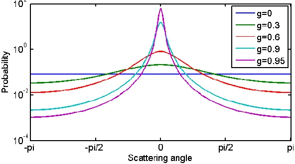
Figure 1-1: Henyey-Greenstein scattering function with different anisotropy factors (g=0,

0.3, 0.6, 0.9, 0.95) ... 4

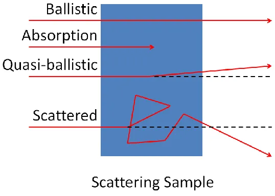
Figure 1-2: Possible photon paths through a scattering sample ... 6

Figure 1-3: Fourier-based ADI ... 11

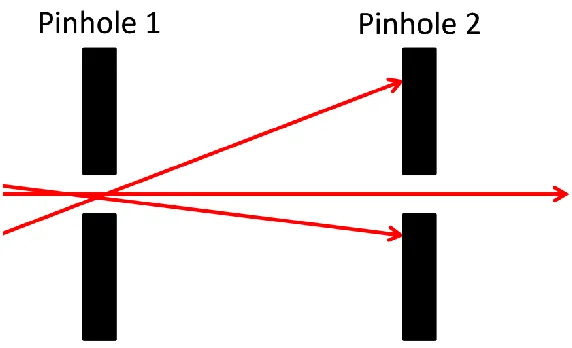
Figure 1-4: Angular domain imaging with two aligned pinholes ... 12

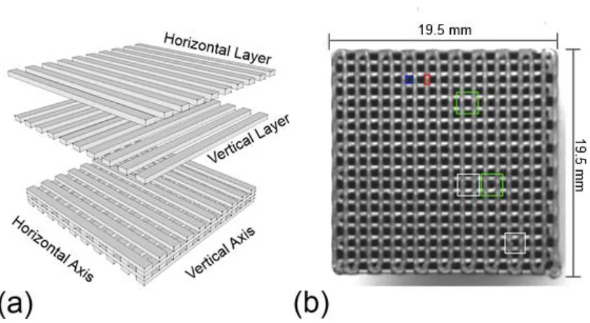
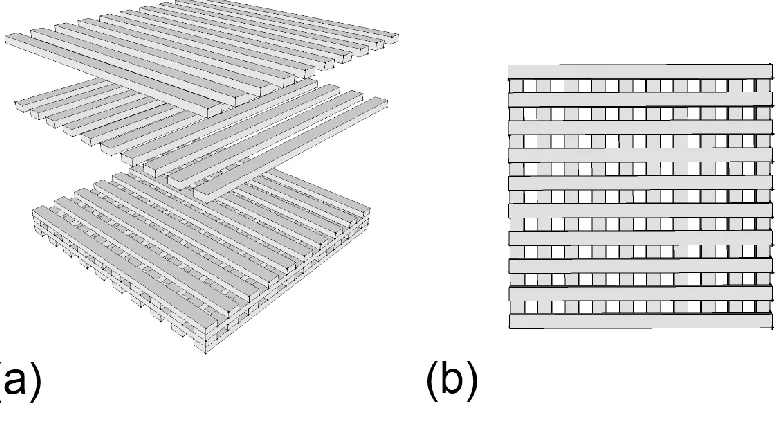
Figure 2-1: Two-dimensional angular filter array made from 3D prototyping. (a) 3D rendering of the AFA construction process with alternating horizontal and vertical parallel walls. Rendering not to scale. (b) Top view photograph of the AFA. Blue outline: channel aperture, red outline: channel wall. White outline, defective channels due to imperfections in plastic deposition. Green outline, channels with rounded edges. ... 37

Figure 2-2: Schematic of the AFA-based ADI setup. Pulsed illumination at 780 nm from a laser (L) was spectrally filtered with a 780 ± 5 nm bandpass filter (SF), restricted with a 1 mm aperture (A) and collimated, expanded, and spatially filtered with collimating optics (C.O.). The collimated light passed through an illumination mask (I.M.), then through the sample (S) and the 2D AFA (AFA). The light was then detected with a CCD camera (C). ... 38

Figure 2-3: Raw AFA images of a 0.9 mm attenuating target in 0.5 % Intralipid® dilution at 1 cm path length collected with a 2D AFA 12 cm in length. (a) No illumination mask, (b) 3 cm illumination mask. Field of view was 8 mm x 8 mm. ... 42

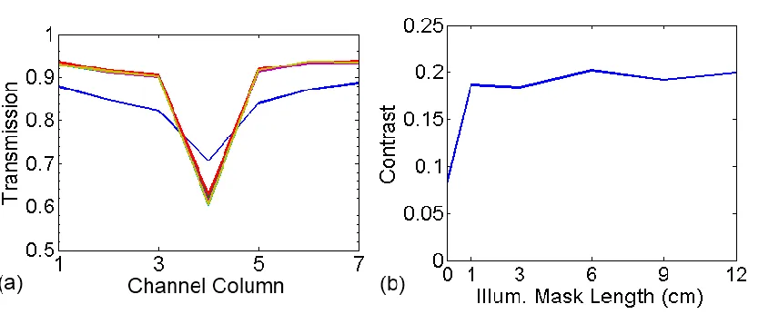
Figure 2-4: Transmission (a) and contrast (b) of a 0.9 mm attenuating target in 0.5 %

Intralipid® dilution at 1 cm path length with a 12 cm 2D AFA and varying

(17)

xvi

no mask, dark green: 1 cm mask, red: 3 cm mask, teal: 6 cm mask, purple: 9 cm

mask, olive green: 12 cm mask. ... 43

Figure 2-5: Transmission (a) and contrast (b) of a 0.9 mm attenuating target in 0.5 %

Intralipid® dilution at 1 cm path length with a 3 cm illumination mask and varying 2D AFA lengths. (a) blue: no AFA, green: 1 cm AFA, red: 3 cm AFA,

teal: 6 cm AFA, purple: 9 cm AFA, yellow: 12 cm AFA. ... 44

Figure 2-6: (a-c) AFA images of a 0.9 mm attenuating target in Intralipid® dilution at 1 cm path length collected with a 15 cm 2D AFA and 3 cm illumination mask after

background subtraction. (a) 0.5% Intralipid®, (b) 0.6% Intralipid®, (c) 0.7% Intralipid® d) Transmission at varying Intralipid® concentrations at 1 cm path length, blue: 0.5% green: 0.6%, red: 0.7%. ... 46

Figure 3-1: Two-dimensional angular filter array fabricated with 3D printing. (a) Exploded

3D rendering of the 2D AFA fabrication details with alternating horizontal and

vertical parallel walls. (b) Top view of the AFA. ... 61

Figure 3-2: Schematic of the ADI setup. Laser: 780 nm pulsed diode laser, Collimating

Optics: Lens-pinhole spatial filter, beam expander and collimator, DLP: 608 x

684 pixel DLP chip (Texas Instruments), Beam Expander: 4x beam expander,

Sample: Cuvette filled with a scattering medium, AFA: 2D Angular filter array,

Camera: CCD Camera with telecentric lens ... 63

Figure 3-3: Images (a, c) and point spread functions (b, d) of a single illuminated channel in

chicken (a, b) and Intralipid® (c, d). (a) Image of a point illumination through 10 mm chicken tissue. FOV = 8 mm x 8 mm (b) Normalized projections of a point

illumination through 6 mm (blue), 8 mm (green), 10 mm (red). (c) Image of a

point illumination through 0.65% Intralipid®. FOV = 8 mm x 8 mm (d) Normalized projections of a point illumination through 0.45% (blue), 0.55%

(18)

xvii

Figure 3-4: Knife edge submerged in Intralipid® (a) 0.65% Intralipid® blue: quasi-ballistic subtraction profile of knife edge averaged from 0.5 mm x 15 mm central region

in the image, red: fitted profile using dual logistic function. (b) Fitted edge spread

functions for the knife edge submerged in 0.45% (blue), 0.55% (green), 0.65%

(red), 0.75% (teal) Intralipid®. ... 71

Figure 3-5: 4 rods (0.2, 0.5, 0.7, 0.9 mm) submerged in (a) 0.6%, (b) 0.7%, (c) 0.75%

Intralipid®. Images are quasi-ballistic images obtained by subtracting the background estimation image from the original image. (d) One-dimensional

profiles obtained by averaging across 1 mm height, blue (0.6%), red (0.7%),

black (0.75%). The field of view was 15 mm x 8 mm. ... 73

Figure 3-6: 4 rods ((a, c, e, g):0.2, 0.5,(b, d, f, h):0.9, 0.7 mm) positioned at the illumination

side of a 1 cm cuvette containing a chicken breast slab. Images (a, b) are

quasi-ballistic images obtained by raster scanning a structured illumination pattern. The

column by column average (c:blue, d:blue) of (a, b) respectively, and the column

by column average of the corresponding breast tissue with the rods removed

(c:red, d:red). Trans-illuminated photographs of the imaging target collected from

the illumination side (e, f) and from the detection (g, h) side of the target. The

field of view was approximately 15 mm x 8 mm. ... 74

Figure 3-7: 0.5 mm rod positioned at the central depth position of a 1 cm cuvette containing a

chicken breast slab. Image (a) is a quasi-ballistic image obtained by raster

scanning a structured illumination pattern. (c) Column by column average of (a).

Trans-illuminated photographs of the imaging target collected from the

illumination side (b) and from the detection (d) side of the target. The field of

view was approximately 15 mm x 8 mm. ... 75

Figure A-1 a) Cartoon of AFA: 80 µm x 80 µm x 2 cm, 200 elements. Channel count and

dimensions are not to scale. b) SEM image (top removed) of a reflection-trapped

(19)

xviii

Figure A-2: Experimental Setup. Laser: Thorlabs 808 nm diode laser, ASL: Aspheric Lens,

P: Pinhole, Collimating Optics: f = -6 mm, f = 100 mm cylindrical lens, Cuvette:

1 cm path length, AFA: element size 80 µm x 80 µm x 2 cm, 200 elements,

Camera: Mightex TCE-1304-U. ... 101

Figure A-3: Imaging target, 4 truncated cones & cylinders. a) top view, b) side view, c) three

dimensional rendering. All measurements are in millimeters. ... 102

Figure A-4: a) Projection of a 0.5 mm graphite rod placed in the center of a 1 cm path length

cuvette, submerged in 0.5% Intralipid®. Red: raw camera signal. Blue dashed: Signal re-binning. Blue: Defective channel removed by averaging signal from

neighboring channels. FOV ~2 mm. b) Projection of graphite rod in (a) displayed

in absorption units. FOV ~1 cm. c) Sample projection of imaging target, slice

#25, ~1.2 mm from cone tips. Target diameter ~360 μm. ... 103

Figure A-5: Sinograms of the imaging target suspended in 0.5% Intralipid® dilution, 60 projections. Field of view is ~1 cm. a) Slice #25 ~1.2 mm from cone tips, target

diameter: ~360 μm b) slice #125 ~9.2 mm from cone tips, target diameter: ~1.4

mm. ... 107

Figure A-6: 2D reconstructions of the 4 cone imaging target suspended in 0.5% Intralipid® dilution at 2 axial slices. a & b) Slice #25 ~1.2 mm from cone tips with filtered

backprojection and iterative reconstruction methods, respectively. c & d) slice

#125 ~9.2 mm from cone tips, reconstructed with filtered backprojection and

iterative reconstruction methods, respectively. ... 108

Figure A-7: 3D reconstruction of the 4 cones imaging target using a) filtered backprojection

and b) iterative reconstruction. The field of view for each slice is ~1 cm x 1 cm.

... 110

Figure B-1: a) Schematic of an AFA (channel count and dimensions not to scale). b) SEM

(20)

xix

Figure B-2: Experimental Setup. Laser: Continuum Surelite OPO, SF: Spectral Filter,

Collimating Optics: f = 125 mm, f = 150 mm, Cuvette: 1 cm path length, AFA:

element size 80 µm x 80 µm x 2 cm, 200 elements, Camera: Mightex

TCE-1304-U. ... 117

Figure B-3: a) Projection of a 0.7 mm graphite rod placed in the center of a 1 cm path length

cuvette, submerged in 0.25% Intralipid®; blue: raw camera signal; black: Signal re-binning; red: Signal with no absorbing target. FOV ~2mm. b) Projection of

graphite rod in (a) displayed in absorption units. FOV ~1.5cm. ... 119

Figure B-4: a) Contrast of a 0.7 mm absorbing rod submerged in 4 levels of scattering at

varying wavelengths. blue: 0.15%; green: 0.2%; red: 0.25%;teal: 0.3%

Intralipid®. b-d) Computed absorption for 0.7 mm absorbing rod at Intralipid® dilutions of (b) 0.2%, (c) 0.25%, (d) 0.3%. blue: 480nm; green 520 nm; red 560

(21)

xx

List of Appendices

A - Three dimensional angular domain optical projection tomography ... 98

(22)

xxi

List of Abbreviations and Symbols

1D, 2D, 3D One, two, three dimensional

ABS Acrylonitrile Butadiene Styrene

ADI Angular domain imaging

AFA Angular filter array

cm Centimeter

CT Computed tomography

CW Continuous wave

DOT Diffuse optical tomography

DRIE Deep reactive ion etching

DTCC 3-diethylthiatricarbocyani

EMCCD Electron multiplied charged coupled device

FDM Fused deposition modelling

fs Femtosecond

FWHM Full width at half-maximum

g Anisotropy factor

HG Henyey-Greenstein

HDMI High-definition multimedia interface

ICG Indocyanine Green

(23)

xxii MEMS Microelectromechanical systems

mm Millimeter

MRI Magnetic resonance imaging

NIR Near infrared

nm Nanometer

OCT Optical coherence tomography

PET Positron emission tomography

ps Picosecond

PTS Photon transport simulator

RTAFA Reflection trapped angular filter array

s Second

SCARA Selective compliance assembly robot arm

SLR Single-lens reflex

SLS Selective laser sintering

SPECT Single-photon emission computed tomography

SVD Singular value decomposition

US Ultrasonogrpahy

UV Ultraviolet

μm Micrometer

(24)

xxiii

Preface

This thesis summarizes the work completed through the duration of my MSc degree

at the University of Western Ontario and Lawson Health Research Institute. This thesis

consists of 4 chapters and 2 appendices. Chapter 1 discusses optical imaging the context of

medical and biological imaging. The background of trans-illumination optical imaging is

presented and the principles behind angular domain imaging and the angular filter array are

described. The chapter concludes with a review of the various approaches, applications, and

developments for angular domain imaging.

Chapters 2 and 3 are based on manuscripts in preparation for submission to

peer-reviewed journals that were written over the course of my degree. The first publication

focused on the design of the novel angular filter array and the optimization of the various

design parameters to obtain images with the highest contrast for a particular imaging task. A

method for structuring the illumination is presented. Chapter 3 describes a resolution analysis

of the angular filter arrays presented in Chapter 2. Chapter 3 also introduces a scanning

mechanism that can be implemented to improve the resolution of the images collected.

Chapter 4 provides a summary and discussion of the project. Chapter 4 also discusses

potential areas where the system can be improved.

Appendices A and B discusses advancements that were made to angular domain

imaging. The experiments performed in Appendices A and B were conducted with the

previous generation one-dimensional angular filter array. Appendix A discusses the

acquisition of three-dimensional images by performing tomography. Appendix B

demonstrates the collection of images at multiple wavelengths using a tunable light source.

The various improvements can be applied to the two-dimensional angular filter array

discussed in Chapters 2, 3, and 4. Both appendices were published as conference

(25)

1

Chapter 1

1

Introduction

This chapter includes a brief introduction of optical-based medical imaging. Angular

domain imaging is an optical imaging modality which illuminates a sample with a light

source, and detects the light exiting the sample with an optical angular filter. In order to

understand angular domain imaging, optical scatter in biological tissue will be described in

detail. The two main approaches to angular domain imaging will then be described in detail.

Various other approaches to optical imaging through scattering media will be discussed as

well.

Angular domain imaging has been studied extensively in the past. Several prototypes

of angular filters have designed and improved upon. Angular domain imaging has also been

combined with other scatter discrimination techniques such as polarization and time domain

imaging. It has been extended to collect three-dimensional images via tomography.

Additionally, multi-spectral and hyper-spectral light sources have been employed to image

spectral targets, and to detect fluorescence through scatter. A brief summary of previous

angular domain imaging studies will be presented.

The objective of this work was to develop a two-dimensional angular filter array to

acquire two-dimensional angular domain images with minimal scanning. Previous angular

domain imaging systems utilized a one-dimensional angular filter, which was inefficient at

acquiring two-dimensional or three-dimensional images. By extending the angular filter to

two-dimensions, two-dimensional images can be acquired significantly faster, and with

minimal scanning. The development of the two-dimensional angular filter represented a

significant hurdle as conventional fabrication technologies used to construct the

one-dimensional angular filter could not easily construct two-one-dimensional objects. This chapter

will discuss the various hurdles associated with the construction of the two-dimensional

angular filter, and it will also discuss the novel fabrication methods used to construct the

(26)

2

their imaging performance was quantified by evaluating the contrast (Chapter 2) and

resolution (Chapter 3) of known absorbing objects embedded in various scattering samples.

This chapter includes background relevant to the understanding of technical details

introduced in Chapters 2 and 3.

1.1 Medical Imaging

The growing need for improving medical diagnoses has necessitated the development

of various medical imaging modalities. Current medical imaging technologies include

magnetic resonance imaging (MRI), x-ray computed tomography (CT), ultrasonography

(US), single photon emission computed tomography (SPECT), and positron emission

tomography (PET). The numerous medical imaging technologies have differing strengths and

capabilities. The various imaging resolutions, contrast mechanisms, sensitivities and

specificities are all factors which are accounted for when selecting an imaging modality for a

specific task.

Generally, MRI provides strong contrast between varying soft tissues. It is capable of

imaging at a large range of depths and resolutions including whole body imaging and small

animal imaging. However, it is often associated with a high cost due to the expensive

equipment, and relatively long acquisition times. CT is capable of generating high contrast

images between bone and soft tissues but it is often incapable of detecting soft tissue

abnormalities. SPECT and PET are capable of functional imaging by imaging radio-labeled

molecules which have been introduced to a subject. However, the resulting images often lack

anatomical detail, and often rely on a second imaging modality to serve as an anatomical

reference. CT, SPECT and PET all utilize ionizing radiation, which can potentially be

harmful if used excessively. Ultrasonography is capable of detecting various tissue densities

in real time. Many tissue abnormalities are often not associated with different tissue

(27)

3

1.2 Optical Imaging

Optical imaging is an emerging medical imaging modality which is currently being

explored as it utilizes a different contrast mechanism from the other commonly used medical

imaging modalities. Optical absorption and scatter provide sources of contrast which cannot

be detected with other imaging modalities. Multispectral imaging can help identify tissue

structures and abnormalities, and potentially measure oxygen saturation or molecular

concentrations. While scatter can often serve as a source of contrast for many optical imaging

modalities, it is a limitation for most optical imaging techniques. Optical scatter often limits

optical imaging to relatively small penetration depths (microns to centimeters). In general,

for purely optical imaging modalities, penetration depth can be increased at the expense of

resolution. For example, ballistic optical imaging can image thin objects at high resolutions,

while diffuse optical tomography can image through thick specimens, but at a reduced

resolution [1,2].

1.3 Light Tissue Interactions

Light travelling through a scattering medium such as a biological tissue sample, can

either pass through unperturbed, or interact with the sample through absorption or scattering

processes. An absorption process is described as the extraction of energy from light by a

molecular species (Figure 1.2, absorption). A scattering process can be described as a change

in the direction of light. Light scattering can be caused by a multitude of processes. For

example, a mismatch in the index of refraction between sub-cellular organelles and the

surrounding cytoplasm can be a source of optical scatter [3].

It is important to note that when light scatters in tissue, the scattering is anisotropic.

Scattering events in tissue tend to be forward directed. The scattering phase function for

tissue is typically modeled after the Henyey-Greenstein function (Eq. 1-1) [4]. The function

models the angular scattering distribution with the use of the average of the cosine of the

(28)

4 2

2 3/2

1 1

( )

4 (1 2 cos( ))

HG

g P

g g



 

 

  whereg 2 ₀cos( )PHG( ) sin( )d



    



_

Eq. 1-1

In the Henyey-Greenstein function, g ranges from [-1,1] and describes the possible

scattering directions from perfect backscattering (g = -1) to isotropic scattering (g = 0) to

complete forward scattering (g = 1). Typical values of anisotropy range from 0.6 to 0.99 for

biological tissues, and are wavelength dependent [5]. The phase functions of varying

scattering values (g) are displayed in Figure 1-1.

Figure 1-1: Henyey-Greenstein scattering function with different anisotropy factors (g=0, 0.3, 0.6, 0.9, 0.95)

While optical imaging can refer to any imaging at wavelengths from ultraviolet to

near infrared, several optical imaging techniques tend to restrict the imaging wavelength to

the tissue optical window, a small range in the near infrared spectrum from 700 to 1100 nm.

Within this wavelength band, intrinsic optical absorbers are at a minimum. Below 700 nm,

hemoglobin is highly absorbing, and beyond 1100 nm, light is absorbed by water. The lack of

intrinsic absorbers in this diagnostic window allows light to penetrate further in the imaging

(29)

5

When a photon of light passes through a scattering sample, there is a possibility that

the photon will not interact with the scattering sample, and pass through the sample

unperturbed (Figure 1-2, ballistic). Unscattered photons, also called ballistic photons, are of

particular interest in optical trans-illumination imaging as ballistic photons can be used to

generate high resolution images. The probability a photon passing through a sample

unscattered is dependent on the scattering nature of the sample, and the thickness of the

sample. Generally, the number of ballistic photons decreases exponentially with thickness.

When imaging through thin tissue samples, (1-2 mm), it becomes difficult to detect ballistic

photons. For tissue samples thicker than 2 mm, virtually no ballistic photons remain [6].

Light scatters through tissue in a forward directed nature. Consequently, when a

sample is illuminated, a small subset of the photons exiting the sample will have undergone a

series of small angle scattering events. These photons are termed quasi-ballistic or snake

photons (Figure 1-2, quasi-ballistic). This subset of photons can potentially be used to

generate higher resolution images compared to purely scattered photons. Theoretically, these

quasi-ballistic photons are able to travel farther through a scattering sample compared to

ballistic photons due to the relaxed nature of their classification. Consequently, when

imaging a relatively thick tissue sample, (2 mm - 2 cm) quasi-ballistic imaging of a sample is

possible, whereas a purely ballistic imaging system will be either unable to generate an

image, or will require a significantly long acquisition time to acquire an image. For many

imaging applications, the tradeoff between resolution and imaging depth or acquisition speed

is often desirable, resulting in considerable interest to develop a quasi-ballistic optical

imaging system.

When a photon scatters within the scattering sample, the path that it travels through

the sample is generally not recoverable. A typical detector will be able to detect the position

at which the photon exits the sample, and a sophisticated detector may even be able to

measure the time the photon travelled within the sample. Multiply scattered light imaging

such as Diffuse Optical Tomography (DOT) utilizes this information to create general

inferences on the probable path of the photon using probability theories and simulated

(30)

6

using multiply scattered light (Figure 1-2, scattered). However, the uncertainty in the images

greatly reduces the potential resolution of an image generated with scattered light.

Figure 1-2: Possible photon paths through a scattering sample

1.4 Overview of Optical Imaging Modalities

Optical imaging techniques can be classified into two groups: purely optical imaging

modalities and hybrid optical imaging modalities. A purely optical imaging modality probes

and detects with light, whereas a hybrid optical imaging modality combines optical imaging

with another method for probing or detecting.

1.4.1 Optical Coherence Tomography

Optical Coherence Tomography (OCT) is currently one of the most advanced optical

imaging modalities. It is commercially available, and it has already been applied extensively

for ophthalmic imaging to obtain images of the retina [7]. OCT relies on optical

interferometry to obtain high resolution superficial images of a target. A low coherence beam

of light is split into a reference beam and a sample beam. The reference beam passes through

an optical path with an adjustable path length, while the sample beam is used to illuminate

(31)

7

and the resulting interference pattern is analyzed. Constructive interference occurs when the

path length of the sample arm is similar to the path length of the reference arm (within the

coherence length of the illumination source). The sample arm is scanned in two axes and the

reference path length is scanned in one axis to generate a three-dimensional image of the

target. Alternatively, a full field illumination scheme can be employed to collect

three-dimensional images by scanning only the reference arm [8]. The short coherence length

serves as a scatter rejection mechanism as only photons that have travelled a similar path

length as the reference arm are imaged. Multiply scattered photons typically travel longer

distances before reaching the detector compared to a non-scattered photon. Due to the

efficiency of the scatter rejection, OCT produces high resolution images (~10 µm typical or

1-2 µm for ultrahigh-resolution OCT) [7,9]. However, it is limited to superficial depths (2-3

mm) due to the lack of ballistic photons at larger depths.

1.4.2 Time domain imaging

Like OCT, time domain imaging discriminates between scattered photons and

unscattered photons by the path length of the photon [10-12]. In time domain imaging, the

path length is measured by the time of flight of a particular photon. Given that the speed of

light is relatively constant through an imaging sample, the time of flight can be used to

deduce the path length of the photon. In time domain imaging, an ultrafast light source (fs) is

combined with an ultrafast detector (fs or ps resolution) to capture images of photons which

have travelled within a given range of path lengths. The detector is controlled by a delay

generator which can vary the time delay of the detector, and correspondingly vary the path

length of the detected photons. When a time gate corresponding to the theoretical time of

flight of an unscattered photon is employed, a near ballistic image will be generated. When

the time gate is relaxed to an extent, a quasi-ballistic image can be obtained. Finally, with a

long time gate, a scatter image can be obtained. A typical time domain ballistic imaging

system is capable of imaging through a thin sample (< 1 mm tissue) with a diffraction-limited

resolution, or through a slightly thicker sample (3.5 mm tissue) in the quasi-ballistic or snake

regime with a resolution of ~200 µm [13]. Using this method, the bone within a human finger

(32)

8

of the equipment required for a typical system. Femtosecond light sources and picosecond

cameras are 10-100 times the cost of a comparable continuous wave (CW) light source and

detector. An optical Kerr cell detection scheme significantly reduces the cost of the detector,

but still requires an ultrafast illumination source.

1.4.3 Diffuse optical tomography

Diffuse optical tomography probes a sample with a series of sources and detectors

[2]. Based on the geometry and scattering properties of the sample, the potential paths of a

large population of photons can be modeled using various photon propagation theories or

simulated via Monte Carlo simulations. A typical DOT system operates in the multiply

scattered regime, where photons undergo several large angle scattering events before

reaching the detector. In this regime, thick tissue samples can be imaged (3 cm – 10 cm). Due

to the use of multiply scattered photons, the resolution of a typical DOT system (~1 cm) is

much larger than an optical ballistic or quasi-ballistic system.

1.4.4 Hybrid optical ultrasound imaging

In addition to purely optical imaging modalities, several hybrid optical imaging

technologies have been developed. Photoacoustic and acousto-optic imaging both combine

ultrasonic imaging with optical imaging [14]. In photoacoustic imaging, a high powered short

pulse of light is used to illuminate a sample. An optically absorbing object embedded within

the sample will then absorb the pulse of light and convert the optical energy to heat. The

rapid heating form the short light pulse will cause a thermoelastic expansion of the target

resulting in the emission of a pressure wave. The pressure wave can then be detected with an

ultrasonic detector, and the position of the target can be triangulated via various

reconstruction algorithms.

Acousto-optic imaging utilizes a continuous wave laser as an illumination source. The

illumination passing through the scattering sample will form a speckle pattern. The sample is

then probed with a focused ultrasound transducer which ultrasonically tags a small region in

(33)

9

the scatterers within the sample, resulting in a modulation of the speckle pattern at the

ultrasound frequency. By analyzing the modulation, the system is able to measure the optical

properties of a small region within the sample [15]. A purely optical imaging system is

unable accomplish this precise sampling of an imaging volume. In both photoacoustic and

acousto-optic imaging systems, the high resolution of ultrasound is combined with the high

contrast of optical imaging.

1.5 Angular Domain Imaging (ADI)

Angular domain imaging is a continuous wave method of quasi-ballistic imaging.

Unlike time domain imaging, it does not require expensive instrumentation, and is relatively

simple to implement. In angular domain imaging, the different types of photons, ballistic,

quasi-ballistic, and scattered are differentiated by the angle at which the photon deviates from

the initial illumination beam. Ballistic photons are unscattered by the imaging sample, and

can therefore be found exiting the sample at the same angle at which it entered the sample.

Quasi-ballistic photons undergo a few forward directed scattering events, and can be found at

small angles with respect to the illumination direction. Finally scattered photons have

undergone multiple large angle scattering events and can be found at large angles with

respect to the illumination direction.

One common design flaw is apparent in angular domain imaging. Quasi-ballistic

photons can be found near the axis of illumination. However photons exiting the sample near

the axis of illumination are not necessarily quasi-ballistic photons. Assuming that the

imaging sample is sufficiently scattering, scattered photons can be found at a wide range of

angles with respect to the axis of illumination. Consequently, a small portion of the scattered

photons will exit the sample at or near the same angle at which they entered the imaging

sample. One major weakness of an angular domain imaging system is the inability to

distinguish between quasi-ballistic photons, and multiply scattered photons which have

scattered back to the axis of illumination.

Angular domain imaging can be performed using one of two methods. The first

(34)

10

use of a lensless collimator. There are subtle differences between the two methods.

Regardless of the method, the effectiveness of the angular filtration is dependent on the

precise positioning of the angular filter in ADI.

1.5.1 Fourier-based ADI

A Fourier-based ADI setup utilizes a converging lens and an aperture to perform

angular filtration [11,16-20]. The aperture is positioned on the back focal plane of the

converging lens. The light emitting from the aperture is then projected onto an imaging

detector. The inclusion of a convex lens allows for the measurement of the Fourier image at

the focal plane of the lens. An aperture positioned at the focal plane acts as a Fourier filter.

The light emitting from the aperture is then transformed back to a real image which is then

imaged with a detector. In the Fourier domain, the spatial frequency of large biological

inclusions is much lower than the spatial frequency of the small random scatterers in a

scattering medium. Consequently, the large biological inclusions will be represented near the

center of the Fourier plane, while the high frequency scatter component will be located far

from the center of the Fourier plane. By selecting an appropriate aperture size, the large

biological inclusions can potentially be distinguished from the scatter photons. Alternatively,

from the perspective of ADI, parallel rays of light will be focused by the converging lens to

the focal point. Non-parallel light will focus elsewhere on the focal plane. A well-positioned

aperture at the focal plane will reject photons that are not parallel with the optical axis

(Figure 1-3). Using ray tracing simulations, the effective acceptance angle of a lens pinhole

(35)

11

Figure 1-3: Fourier-based ADI

One interesting limitation of the lens aperture method to ADI is the scatter rejection

of a pinhole is linked directly with the Fourier frequency. By using a smaller pinhole, the

system will conceivably reject more high frequency scattered light. However, the rejection of

high frequency scattered light also imposes a restriction on the potential resolution of the

image as the high frequency Fourier component may be required to form a faithful image. A

second limitation of the lens aperture method is the use of a lens in the filtration step. A lens

is commonly associated with various aberrations (e.g. spherical, chromatic), and as a result

cause deviations between the theoretical and experimental performance. In addition,

chromatic aberrations may limit the ability to image at multiple wavelengths of light,

potentially preventing multi-spectral or hyper-spectral imaging.

1.5.2 Lensless ADI

A lensless collimator can refer to a variety of designs. The simplest collimator

consists of a pair of aligned pinholes separated by a distance (Figure 1-4). The first pinhole

serves to restrict the light entering the collimator to a small aperture, while the second

pinhole passes only light which has travelled in the axis of the collimator. The acceptance

angle of this collimator is dependent on the size of the pinhole as well as the spacing between

the pinholes. A larger pinhole and a shorter spacing will result in a larger acceptance angle,

while a smaller pinhole and a larger spacing will result in a smaller acceptance angle. This

simple design only allows for the imaging of a single point. Consequently, a two-dimensional

(36)

12

Figure 1-4: Angular domain imaging with two aligned pinholes

In order to parallelize the acquisition process, a series of pinholes can be used instead

of a single pinhole. To prevent crosstalk between the pinholes, a lattice structure must be

placed between the two arrays of pinholes. This design is the basis of a Söller collimator in

x-ray imaging, or an Angular Filter Arx-ray (AFA) in optical imaging [21]. Much like the pair of

pinholes, the acceptance angle of the AFA is based on the aspect ratio of the optical channel.

1.5.3 ADI simulations

Angular domain imaging using a lensless angular filter has been extensively studied

by two research groups: the Chapman group at Simon Fraser University and our group, the

Carson group, at the Lawson Health Research Institute. Previously, Monte Carlo simulations

were conducted by the Chapman group to study the theoretical performance of an

angle-based scatter rejection imaging method [22,23]. Monte Carlo simulations are considered the

gold standard for simulating photon transport through a scattering medium as it is capable of

simulating arbitrary complex geometries. The major drawback to the Monte Carlo method is

the significant computational resources required to generate a statistically acceptable result.

Previous simulations were conducted on a custom software package, Photon Transport

Simulator (PTS), which was designed to model the effects of the various angular filters. In

PTS, the photon transport modeling through a scattering medium was based on a previous

(37)

13

Extensive simulations were conducted to test the theoretical performance of an ADI

system. The first simulation tested the fundamental basis of ADI, and the principle of angular

selection as a quasi-ballistic photon discriminator. A typical quasi-ballistic photon will

exhibit a shorter path length through a scattering sample compared to a multiply scattered

photon. A Monte Carlo simulation was performed to examine whether smaller angular

deviations at the exit face of a sample corresponded to photons with shorter path lengths. The

results indicated that for intermediate scattering levels, a smaller acceptance angle

corresponded to a smaller mean photon path length. At higher scattering levels, this effect

was not observed, suggesting that there is a fundamental limit of ADI and ADI systems are

expected to fail when the scattering of the sample is beyond a particular limit [22]. The

simulation conclusions were consistent with the results of a separate study which

demonstrated that photons exiting the sample at smaller angles are related to the early

arriving photons in a time domain system. In this study, the temporal point spread function

was observed to decrease when a smaller acceptance angle was utilized. Measurements were

conducted with various combinations of Intralipid® concentration and optical cell thicknesses, with the product of the concentration and the length held constant at the equivalent of 2%

Intralipid® and 10 mm cell thickness [11]. Intralipid® is a lipid emulsion that serves as a convenient phantom to simulate optical scatter in biological tissue [25]. In a separate study,

projection images of a target embedded in a scattering medium were collected with a

collimated light beam. Image contrast was found to be greatly improved with the addition of

a Fourier angular gate after the scattering medium [10]. Another study reported the imaging

of 0.25 mm black bars submerged in a 5.5 cm thick optical cell filled with 2.5% Intralipid® with the use of a Fourier gate [16].

A second simulation was conducted by the Chapman group to test the theoretical

resolution of a micro-channel array [22]. One concern of the micro-channel array was the

potential relation between channel size and the resolution of the imaging system. A Monte

Carlo simulation was conducted where an object smaller than the size of the channel was

imaged through a scattering medium. The results indicated that the object was clearly

resolvable for lower scattering levels. Higher scattering levels were unable to be tested with

(38)

14

indicate that the resolution of an AFA image is dependent on the resolution of the detector

(camera) and not dependent on the size of the channels.

A third simulation conducted by the Chapman group tested the theoretical acceptance

angle for an individual AFA channel. When a photon of light strikes the wall of the AFA, it

can either be absorbed by the AFA or reflected. The probability of reflection increases as the

angle of incidence with the wall increases (i.e. a photon that strikes the wall at a glancing

angle has a higher probability of reflecting compared to a normally incident photon). Internal

reflections increase the effective acceptance angle of an AFA compared to the theoretical

acceptance angle of that AFA. The theoretical acceptance angle can be computed

geometrically (Eq. 1-2) and is representative of the acceptance angle of the AFA under the

assumption that all photons striking the walls of the channels attenuate. For a typical angular

filter with an aspect ratio (collimator length / collimator diameter) of 200, the theoretical

acceptance angle is 0.28°. Due to internal reflections, simulation studies show that the

acceptance angle for a silicon-based AFA with an aspect ratio of 200 is approximately 2.3º

[23].

1 collimator diameter

tan ( )

collimator length _ 

Eq. 1-2

A fourth simulation was conducted by the Chapman group to test the effect of

aperture size on acceptance angle. For a micro-channel based collimator, the size of the

aperture can potentially be changed without changing the acceptance angle by increasing the

length of the channel correspondingly. A simulation was conducted where the aspect ratio of

the channel was held constant at 200, while the diameter of the channel was varied from 10

µm to 100 µm. The simulation results demonstrated that the acceptance angle of the

micro-channel array was constant for the various micro-channel diameters, suggesting that the acceptance

angle was indeed dependent on the aspect ratio of the channels and was not dependent on the

size of the channel itself. The results also indicated that for smaller channels (< 100 µm

diameter), the overall efficiency of the channel was decreased. This effect was attributed to

diffraction effects from smaller sized channels. The results suggest that to optimize AFA

(39)

15

1.6 Previous AFA design

Several collimator designs that fit the AFA description have been described

previously in the literature [21]. However, the specifications and fabrication methods are

often omitted in these studies. One silicon-based AFA design has been replicated in multiple

studies by the Chapman and Carson groups [19,22,23,26-43]. The silicon-based AFA design

utilizes MEMS-based fabrication techniques to create a series of channels in a silicon wafer.

The first design was constructed using a chemical isotropic etchant. The second design

replaced the chemical isotropic etchant with a Deep Reactive Ion Etching (DRIE) machine

for added control during the etching process.

1.6.1 Silicon AFA fabrication process

The silicon-based AFAs were constructed by first allowing the growth of a layer of

silicon dioxide (SiO2) on a silicon wafer to act as a masking layer. A photoresist was then

spin coated on the wafer and exposed with a UV lithography process to transfer a mask

pattern onto the photoresist. The developed photoresist was used as a mask to etch the

underlying SiO2 layer. The patterned SiO2 layer was then used as a mask for etching the

silicon wafer via a chemical isotropic etchant or a DRIE machine. Finally, the SiO2 layer was

removed, leaving a series of micro-channels embedded in a silicon wafer. The wafer was

then diced to expose the entrance and exit faces of the micro-channels. A second silicon

wafer was then positioned on top of the micro-channels to enclose the top surface of the

channels.

1.6.2 Chemically etched AFAs

The chemically etched AFAs resulted in a series of micro-channels with a

circular cross section due to the isotropic nature of the etchant. In this design, the

semi-circular channels each had a radius of 25 µm and a length of 1 cm. Neighboring channels

were spaced periodically at 100 µm. The acceptance angle of the channels can be computed

geometrically under the assumption that no internal reflections occur. For this design, the

(40)

16

chemical etching process was the poor reproducibility of the fabrication. The etch rate was

sensitive to the agitation of the sample container. In addition, the resulting semicircular

channel cross section suffered from a low fill factor due to the changing wall thicknesses

between channels [34].

1.6.3 Deep Reactive Ion Etching AFAs

One method of improving the fill factor was changing the fabrication process to etch

micro-channels with a square cross section. DRIE allows for anisotropic etching of the

silicon wafer. In addition, the DRIE method was highly reproducible and resulted in channels

with excellent uniformity across the entire area of the silicon wafer. By utilizing the DRIE

method, the sizes of the micro-channels were highly customizable. AFAs with a wide range

of channel sizes (20 µm x 20 µm to 80 µm x 80 µm) and channel lengths (0.5 cm to 2.0 cm)

were constructed and a series of experiments were conducted by the Carson group to evaluate

the contrast of each AFA [43]. The DRIE method was determined to be superior to the

previous isotropic etching method for reproducibility and AFA design.

1.6.4 Internal reflections

In addition to highly reproducible fabrication, the DRIE method allowed for another

improvement over the chemical etching method. One concern of the AFA collimator was the

potential for photons to strike the walls of the channels at glancing angles, and reflect. An

internal reflection will increase the effective acceptance angle of the channel, and result in an

angular filter with poorer contrast and resolution performance. In previous studies by the

Chapman group and the Carson group, two main approaches were used to attempt to

minimize the internal reflections within the AFA.

The first approach was to deposit a thin layer of optically absorbing material on the

surface of the micro-channels to improve the absorption of the photons that strike the walls

of the AFA. A carbon arc evaporator system was first used to deposit a thin layer (30 - 40 nm)

on the surface of the AFA. Preliminary studies were conducted where successive images of

(41)

17

rotations allowed for the measurement of the internal reflections. The rotation studies

indicated that the internal reflections were subdued to an extent when a carbon layer was

deposited on the AFA however this result was never quantified by the author of the study

[27]. One drawback of the evaporation method was the high level of debris generated,

leading to the partial or full occlusion of several AFA tunnels. This deposition method was

later improved by the Carson group with the use of a carbon sputter deposition process

instead of an evaporation deposition process [42]. The sputter deposition method provided

higher uniformity and excellent adhesion.

The second approach to minimize internal reflections was to reduce the angle of

incidence of photons striking the walls of the AFA. This was accomplished by altering the

smooth surface of the AFA walls. In the first design, the surface of the AFA was roughened

by including an additional etching step to the fabrication process. The AFA was wet etched

using a NH4OH solution [27]. Preliminary experiments suggested that the roughened walls

decreased the internal reflections within the channels, but this effect was not quantified. One

weakness of the etching process was the uneven etching across the entire AFA. This problem

was addressed in the second design of the wall roughening process. In the second design by

the Carson group, a periodic wall pattern was incorporated into the lithography mask [40,42].

Ridges 2.5 µm tall were positioned at 20 µm intervals along the length of the AFA channels.

The new AFA design was termed the Reflection Trapped AFA or (RTAFA). The ridges were

designed to reduce the angle of incidence of any photon striking the walls of the channel to

promote the absorption of the scattered light. The ridges also contained the scattered photons

within the AFA to an extent. The new RTAFA design was demonstrated to improve the

contrast of a resolution target suspended in a scattering medium compared to a conventional

AFA design. For example, a 50% increase in image contrast was observed when utilizing a

60 µm x 60 µm x 1.5 cm RTAFA over a conventional AFA when imaging through a 0.3%

Intralipid® dilution at a 2 cm optical path length [40]. Due to the nature of the fabrication process, the RTAFA only exhibited patterned vertical walls. The patterning of the top and

bottom surfaces of the square channels would require additional lithography masks, and

(42)

18

1.7 ADI Illumination sources

AFA-based ADI has been demonstrated with various illumination sources. For

trans-illumination imaging, three main qualities are considered. The first is the imaging

wavelength. Several biological targets are detectable at specific wavelengths. Much of the

preliminary work in ADI has been conducted with tissue mimicking phantoms and

wavelength independent targets. Consequently much of the early work in ADI was conducted

at a multitude of arbitrary wavelengths. One particular study of interest by the Chapman

group evaluated the performance of the ADI system at three wavelengths in the visible and

near infrared spectrum [37]. Several attempts have also been made to combine ADI with a

hyper-spectral light source. A study was conducted by the Carson group, with a Quartz

Tungsten Halogen lamp, which emits light over a continuous range of wavelengths

simultaneously [39]. An additional study published by the author was conducted with a

wavelength tunable light source (Appendix B) [29].

In trans-illumination imaging, the collimation of the illumination source generally

improves the quality of the resulting images [20,44]. Typically laser light sources can be

highly collimated, and are suitable for ADI. A lamp typically generates light from a large

filament, resulting in a source that is difficult to collimate efficiently.

In trans-illumination imaging, the geometry of the illumination source is also an

important factor to consider. Generally, extended light sources perform poorer when

compared to a scanning point light source. This is due to the potential for light to scatter into

a neighboring area. A raster scanning point illumination system will be able to account for

optical smearing due to scatter, while a full field image collects all the data simultaneously,

and is therefore unable to intrinsically remove the excess scatter. In a previous study

performed by the Chapman group, when a sample was illuminated with a line of light, image

(43)

19

1.8 Previous ADI studies

1.8.1 Hybrid ADI systems

ADI has been studied extensively over the past decade. Several attempts have been

made to combine ADI with a complimentary scatter rejection method to improve the

performance of ADI at higher scattering levels. The Carson group examined the

depolarization of light as a method to distinguish between ballistic and multiply scattered

photons [38]. In addition to polarization gating, the Carson group utilized time gating in

conjunction with ADI. An ultrafast pulsed laser (270 ps) was combined with a picosecond

gated camera to provide time gating alongside the angular gating from ADI. Contrast was

demonstrated to improve for a given scattering level, however the system was unable to

image at scattering levels beyond the limit for ADI-only systems [40].

1.8.2 Background scatter estimation

When imaging near the scattering limit with ADI, it is possible to improve the

contrast of images by estimating the background scatter signal. A typical ADI image contains

signal from two components, a quasi-ballistic component and a background scatter

component. The quasi-ballistic component is the information containing component, and the

source of contrast in the image. The background scatter is present due to the imperfect nature

of angular filtration based imaging at high scattering levels. At high scattering levels,

multiply scattered photons can potentially scatter back into the axis of illumination and

contribute to a background signal in the image. The background signal in an image reduces

image contrast. One method of improving the image contrast is to estimate the background

signal through various methods, and then subtract the background signal from the original

image to obtain a better approximation of a quasi-ballistic image. In the combined angular

and polarization gating experiment mentioned previously, the background scatter was

estimated by obtaining an image with the analyzer and the polarizer positioned in the crossed

position. The crossed polarization image was not expected to contain any quasi-ballistic

(44)

20

hybrid time-angular domain imaging system mentioned previously, a scatter estimation

image was obtained by imaging the sample at a late gate delay where no quasi-ballistic

photons were expected to be detected [31]. In ADI systems described by the Carson group,

the scattered component was measured by introducing an optical wedge into the illumination

path. An optical wedge was expected to deviate the illumination by an angle larger than the

acceptance angle of the AFA. As a result, when an image was collected with a scattering

sample, the image was expected to contain only the scattering component [38]. The principle

of scatter estimation has been applied to various other trans-illumination imaging systems

including the use of a differentiometer to measure the difference between on axis and off axis

light [45] and the use of a diffuser in the illumination path to destroy the collimation of the

light, and obtain a scatter only image [46,47].

1.8.3 Deep illumination ADI

While some ADI studies have been focused on improving the imaging performance

of ADI, other studies have been focused around finding potential applications for ADI. One

example involves a significant change in the imaging setup from a trans-illumination imaging

system to a reflection-based imaging system [36,48]. One of the main drawbacks of

trans-illumination ADI is the limitation of sample thickness. ADI has only been successful at

imaging samples with a small optical thickness (6 reduced mean free paths) [40]. This

corresponds to a tissue thickness of approximately 6 mm, and significantly limits the

application of ADI in a clinical setting. By switching the setup to collect reflected images,

the ADI system will be able to capture images of samples up to 3 mm below the surface of a

sample. This may potentially find applications in dermatology or endoscopy. Light scattering

in tissue has been described to be forward directed. However, there is a small portion of light

that undergoes backscattering. The backscattering was used as an illumination source for

deep illumination ADI. Using this ADI setup, two-dimensional absorbing targets were

(45)

21

1.8.4 Tomographic ADI

Optical trans-illumination imaging is similar in principle to x-ray planar imaging.

X-ray planar imaging has been successfully extended to collect three-dimensional images via

computed tomography. Optical tomography has already been previously demonstrated with

time domain imaging [49]. As a result, a natural extension of ADI was to collect tomographic

images of a sample and to reconstruct the images to obtain three-dimensional images of a

sample. In an initial study conducted by the Carson group, two attenuating rods of 0.9 mm

diameter were submerged in a 2 cm optical cuvette filled with a 0.3% Intralipid® dilution. The two rods were imaged at 200 projections and successfully reconstructed. The author

conducted a follow-up study where a series of four cylindrical rods ranging from 0.2 mm to

0.9 mm diameter suspended in a 0.6% Intralipid® dilution at 1 cm path length were imaged and successfully reconstructed with 60 projections. Two hex keys 1.2 mm wide and 2 mm

wide were also reconstructed when placed in the same scattering solution. Finally a 2 cm

diameter grape was imaged, and the seeds of the grape were successfully reconstructed [30].

The author conducted another study which involved the collection of three-dimensional

angular domain images via rotation and scanning. A custom resolution target with four

truncated cones varying in diameter from 1.2 mm to 0.2 mm was constructed and positioned

in a scattering sample. The structure was successfully reconstructed in three dimensions [32].

1.8.5 Fluorescence ADI

While conventional ADI utilizes absorbing targets within a scattering medium as

sources of contrast, a fluorescent target can be used as an optical source within the scattering

sample itself. In one study conducted by the Carson group, two 1.2 mm diameter tubes filled

with 3-diethylthiatricarbocyanin (DTTC, 20 µM) were positioned at a depth of 1 mm in a

cuvette filled with 1% Intralipid® dilution. The tubes were successfully resolved when using an AFA. The tail of a hairless SKH1 mouse (6 weeks old) was also imaged after the injection

of an optical bone marker (IRDye® 800CW BoneTag). The vertebrae of the mouse were resolved [35]. A second study conducted by the Carson group demonstrated the possibility of