CHAPTER 4 Volatility and Correlation : Measurement, Models and Applications

Full text

(1)Risk Management and Analysis: Measuring and Modelling Financial Risk (C. Alexander, Ed) Wileys, (1998) CHAPTER 4. Volatility and Correlation : Measurement, Models and Applications Carol Alexander, University of Sussex UK. 4.1 Introduction The most widely accepted approach to ‘risk’ in financial markets focuses on the measurement of volatility in certain returns distributions.1 The volatility of portfolio returns depends on the variances and covariances between the risk factors of the portfolio, and the sensitivities of individual assets to these risk factors. In linear portfolios, sensitivities are also measured by variances and covariances. So the primary objective of this chapter is to account for the standard methods of estimating and forecasting covariance matrices. The practical and theoretical advantages and limitations of each method is discussed in detail. Later it is shown how to employ them effectively in value at risk systems, capital allocation models, investment management and the pricing and hedging of derivative products. The chapter concludes with a short review of other methods for measuring market risk: downside risk and regret, expected maximum loss, and cointegration. What is volatility? A standard non-parametric definition is that x is 'more volatile' than y if P(x>c) > P(y>c) for all c. So if y is a time series it becomes more volatile when P(yt+1>c) > P(yt>c) for all c. But when y has a symmetric distribution, such as a normal distribution, this occurs if and only if σ. 1. Returns are given by the relative change in prices (or rates) over a fixed holding period h. The return at time t is given by (Pt - Pt-h)/Pt-h which, for small h, is well approximated by lnPt - lnPt-h . Value at Risk is, however, based on the volatility of a portfolio’s change in market price (the profit and loss, P&L). Both returns and P&L are generally stationary (mean reverting) variables. But some confusion may be caused by the term ‘price volatility’, since prices (or rates) are random walks in efficient markets, and hence have infinite (unconditional) variance..

(2) Risk Management and Analysis: Measuring and Modelling Financial Risk. 2. (C. Alexander, Ed) Wileys, (1998) 2. 2 t+1 > σ t where σ t denotes the conditional variance of y. However, variance is not 2. 2. standardized. If we were to plot a term structure of variances, across different maturities, variance would simply increase with the holding period of returns. So volatility is usually quoted as an annualised percentage standard deviation: volatility at time t = (100 σt √A) %. (1). where A denotes the number of observations per year. We do this so that volatilities of different maturities may be compared on the same scale - as the variance increases with the holding period, so the annualising factor decreases. In this way, volatilities are standardized. If one takes two associated returns series x and y - returns on two Gilts for example - we can calculate their correlation as CORR (x ,y) = COV(x ,y) / √V(x) √V(y). (2). that is, ρxy = σxy / σx σy. (3). Note that joint stationarity3 is necessary for the existence of correlation, and that it is the exception rather than the rule. Two arbitrary returns series, such as a Latin American Brady bond and a stock in the FTSE 100, should be unrelated and are not likely to be jointly stationary, so correlations between these two time series do not exist. Of course, one can calculate a number based on the correlation formulae given in this chapter, but it does not measure unconditional correlation unless the two series are jointly stationary. In such cases 'correlation' is found to be very unstable. Correlation estimates will jump about a lot over time - a sign of non-joint stationarity.. We use the notations V(.) and σ2 interchangeably, similarly COV(x,y) and σxy . The standard deviation is the square root of the variance. Conditional and unconditional variance are explained in section 4.3.1.. 2. 3. Loosely speaking, this means that not only are the two individual returns series stationary (mean reverting) , but their joint distribution has stationarity properties such as constant autocorrelations..

(3) Risk Management and Analysis: Measuring and Modelling Financial Risk. 3. (C. Alexander, Ed) Wileys, (1998). Correlation does not need to be annualised, as does volatility, because it is already in a standardised form: correlation always lies between -1 and +1. A negative value means that returns tend to move in opposite directions and a positive value indicates synchronous moves in the same direction. The greater the absolute value of correlation, the greater the association between the series. 4 Volatilities and correlations are just standardized forms of the variances and covariances between returns, so the information necessary to measure portfolio risk is usually summarized in a covariance matrix. Based on a set of n returns series y1, ….. yn , this is a square, symmetric matrix of the form V ( y1 )    COV ( y 1 , y 2 )  COV ( y 1 , y 3 )  ...    COV ( y 1 , y n ). COV ( y 1 , y 2 ) ... V ( y2 ) ... COV ( y 2 , y 3 ) V ( y 3 ) ... ... ... .... ... COV ( y 1 , y n )   ... COV ( y 2 , y n )  ... COV ( y 3 , y n )   ... ...   ... V ( yn ) . The next two sections of this chapter describe the two most commonly used methods of estimating and forecasting covariance matrices in financial markets. Section 2 assesses the moving average volatility and correlation estimation methods that are most financial institutions use today: the equally weighted 'historic' method and the exponentially weighted moving average method. Section 3 gives an overview of the huge technical literature on GARCH modelling in finance and section 4 covers implied volatility and correlation forecasts, their use in trading being covered elsewhere in this book (chapter 18). Section 5 surveys the use of volatility and correlation forecasts in risk management, with particular emphasis on value at risk (VAR) models. The last section of this chapter covers certain special issues, such as estimating volatilities from ‘fat-tailed’ distributions using normal mixtures, evaluation of the accuracy of different models, and new directions, such as ‘downside risk’ measures and cointegration. 4. It is important to bear in mind that returns series can be perfectly correlated even when the prices are in fact moving in opposite directions. Correlation only measures short-term co-movements in returns, and has little to do with any long-term co-movements in prices. For the common trend analysis in prices, rates or yields the technique of cointegration offers many advantages, and this is reviewed in the last section of the chapter..

(4) Risk Management and Analysis: Measuring and Modelling Financial Risk. 4. (C. Alexander, Ed) Wileys, (1998). 4.2 Moving Averages A moving average is an arithmetic average over a rolling window of consecutive data points taken from a time series. Moving averages have been a useful tool in financial forecasting for many years. For example, in technical analysis, where they exist under the name of 'stochastics', the relationship between moving averages of different lengths can be used as a signal to trade. Traditionally they have also been used in volatility estimation. Usually volatility and correlation estimates are based on daily or intra-day returns, since even weekly data can miss some of the turbulence encountered in financial markets. Moving averages of squared (or cross products) of returns are estimates of variance (or covariance). These are converted to volatility and correlation as described above, or employed in a covariance matrix for measuring portfolio variance. 4.2.1 'Historic' Methods This section describes the uses and misuses of the traditional ‘historic’ volatility and correlation forecasting methods. Recent advances in time series analysis allow a more critical view of the efficiency of these methods, and they are being replaced by exponentially weighted moving average or GARCH methods in most major institutions today.. (. The n-period historic volatility at time T is the quantity 100 σ$T. ). A % where A is the number of. returns rt per year and σ$. 2 T. =. t = T −1. ∑r. t =T −n. t. 2. /n. (4). Thus σ$T is the unbiased estimate of standard deviation over a sample size n, assuming the mean is zero.5. It is usual to apply moving averages to squared returns rt2 (t = 1,2,3,....n) rather than squared mean deviations of returns (rt - r )2 where r is the average return over the data window. Although standard statistical estimates of variance are based on mean deviations, empirical research on the accuracy of variance forecasts in financial 5.

(5) Risk Management and Analysis: Measuring and Modelling Financial Risk. 5. (C. Alexander, Ed) Wileys, (1998). 'Historic' correlations of maturity n are calculated in an analogous fashion: if x and y are two returns series, then n-period historic correlations may be calculated as6 t = T −1. rT. =. ∑x y t. t = T −n t = T −1. ∑. t = T −n. 2. xt. t. t = T −1. ∑y. t =T −n. (5) 2. t. Traditionally, the estimate of volatility or correlation over the last n periods has been used as a forecast over the next n periods. The rationale for this is that long-term volatility predictions should be unaffected by ‘volatility clustering’ behaviour, and so we need to take an average squared return over a long historic period - but short-term volatility predictions should reflect current market conditions, whether volatile or tranquil, which means that only the immediate past returns should be used. However, when we examine the time-series properties of ‘historic’ volatilities and correlations we see that they have some undesirable qualities: A major problem with equally weighted averages is that extreme events are just as important to current estimates whether they occurred yesterday or a long time ago. Even just one unusual return will continue to keep volatility estimates high for exactly n days following that day, although the underlying volatility will have long ago returned to normal levels. Thus volatility estimates will be kept artificially high in periods of tranquillity, and they will be lower than they should be during the short bursts of volatility which characterise financial markets.7. markets has shown that it is often better not to use mean deviations of returns, but to base variances on squared returns and covariances on cross products of returns (Figlewski, 1994, Alexander and Leigh, 1997). 6. Again, assuming zero means is simpler, and there is no convincing empirical evidence that this degrades the quality of correlation estimates and forecasts in financial time series 7. For this reason I suggest removing extreme events from the returns data before the moving average is calculated. This will give a better ‘everyday’ volatility estimate, for example, in VAR models. For stress testing portfolios, these extreme events can be put back into the series - indeed they could even be bootstrapped back into the series for more creative stress testing..

(6) Risk Management and Analysis: Measuring and Modelling Financial Risk. 6. (C. Alexander, Ed) Wileys, (1998). Figure 1 illustrates equally weighted averages of different lengths on squared returns to the FTSE. Daily squared returns are averaged over the last n observations for n= 30, 60, 120, 240, and this variance is transformed to an annualized volatility in figure 1. Note that the one-year volatility of the FTSE jumped up to 26% the day after Black Monday and it stayed at that level for a whole year because that one, huge squared return had exactly the same weight in the average. Exactly one year after the event the large return falls outs of the moving average, and so the volatility forecast returned to its normal level of around 13%. In shorter term equally weighted averages this ‘ghost feature’ will be much bigger because it will be averaged over fewer observations, but it will last for a shorter period of time.. Figure 1: Historic Volatilities of the FTSE from 1984 to 1995, showing 'ghost features' of Black Monday and other extreme events 70 60 50 hist30 40. hist60 hist120. 30. hist240. 20 10. 2623. 2509. 2395. 2281. 2167. 2053. 1939. 1825. 1711. 1597. 1483. 1369. 1255. 1141. 1027. 913. 799. 685. 571. 457. 343. 229. 1. 115. 0. Ghost features are even more of an issue with equally weighted moving average correlation estimates, where they can induce an apparent stability in correlations. It may be that ‘instantaneous’ correlations are very unstable, because the two returns are not jointly stationary. But whatever the true properties of correlations between the two returns series, the longer the averaging period, the more stable will moving average correlations appear to be. It may also be.

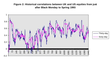
(7) Risk Management and Analysis: Measuring and Modelling Financial Risk (C. Alexander, Ed) Wileys, (1998). that, by some fluke, the series both have large returns on the same day. This will cause a ghost feature in correlation, making it artificially high for the n periods following that day. Even with two closely related series such as the FTSE 100 and the S&P 500, we will obtain correlation estimates which appear more stable as the averaging period increases. This point is illustrated in figure 2, where correlations between the two equity indices are shown for a 60-day averaging period, compared with the 30-day period. Stability of correlation estimates increases with the averaging period, rather than being linked to the degree of joint stationarity between the variables, because the equally weighted moving average method is masking the underlying nature of the relationship between variables. Thus we could erroneous conclude that correlations are ‘stable’ if this method of estimation is employed.. Figure 2: Historical correlations between UK and US equities from just after Black Monday to Spring 1993 1 0.8 0.6 Thirty-day 0.4. Sixty-day. 0.2. 1441. 1369. 1297. 1225. 1153. 1081. 1009. 937. 865. 793. 721. 649. 577. 505. 433. 361. 289. 217. 145. 73. 1. 0 -0.2. Equally weighted moving averages should be used with caution, particularly for correlation, on the grounds of these ghost features alone. But there is another, finer point of consideration. Perceived changes in volatility and correlation can have important consequences, so it is essential. 7.

(8) Risk Management and Analysis: Measuring and Modelling Financial Risk. 8. (C. Alexander, Ed) Wileys, (1998). to understand what is the source of variability in any particular model. In the 'historic' model, all variation is due only to differences in samples: a smaller sample size yields a less precise estimate, the larger the sample size the more accurate the estimate. So a short period moving average will be more variable than a longer moving average. But whatever the length of the averaging period we are still estimating the same thing: the unconditional volatility of the time series. This is one number, a constant, underlying the whole series. So variation in the n-period historic volatility model, which we perceive as variation over time, is actually due to sampling error alone. There is nothing else in the model that allows for variation. There is no estimated stochastic volatility model in any moving average method - they are simply estimates of unconditional moments, which are constants. 8 The estimated series does change over time, but as the underlying parameter of interest is a constant variance, all the observed variation in the estimate is simply due to sampling variation. The 'historic' model is also taking no account of the dynamic properties of returns, such as autocorrelation. It is essentially a 'static' model which has been forced into a timevarying framework. So, if you 'shuffle' the data within any given n-period window, you will get the same answer, provided of course for correlation the two returns series are shuffled 'in pairs'. 4.2.2 Exponentially Weighted Moving Averages The 'historic' models explained above weight each observation equally, whether it is yesterdays return or the returns from several weeks or months ago. It is this equal weighting that induces the 'ghost features', which are clearly a problem. An exponentially weighted moving average (EWMA) places more weight on more recent observations, and this has the effect of eliminating the problematic 'ghost features'. The exponential weighting is done by using a ‘smoothing constant’ λ: the larger the value of λ the more weight is placed on past observations and so the smoother the series becomes. An n-period EWMA of a time series x is defined as. 8. This is a limitation of moving average methods. When the estimation method also gives a model for stochastic volatility (as it does, for example, in GARCH models) the stochastic volatility model has very useful applications for pricing and hedging (see sections 4.5.2 and 4.5.3).

(9) Risk Management and Analysis: Measuring and Modelling Financial Risk. 9. (C. Alexander, Ed) Wileys, (1998). x t −1 + λ x t −2 + λ x t − 3 + ..... + λ. n −1. 2. 1+λ. + λ2 + ...... + λn −1. x t −n. (3). Since the denominator converges to 1/(1-λ) as n → ∞, an infinite EWMA may be written (1 − λ ). ∞. ∑λ. i −1. i =1. x t − i −1. (4). It is an EWMA that is used for volatility and correlation forecasts in JP Morgan and Reuter’s RiskMetrics . The forecasts of volatility and correlation over the next day are calculated by taking λ=0.94 and using squared returns r2 as the series x in (7) for variance forecasts and cross products of two returns r1r2 as the series x in (7) for covariance forecasts. Note that the same value of λ should be used for all variances and covariances in the matrix, otherwise it may not be positive semi definite (see JP Morgan, 1996) . In general this type of EWMA behaves in a reasonable way - see Alexander and Leigh, 1997 for an evaluation of their accuracy. In fact, an EWMA on squared returns is equivalent to an IGARCH model (see section 4.3.2). To see this, consider equation (7) : σ$t2. = (1 − λ ). ∞. ∑λ. i −1. i =1. rt 2−i −1. This may be re-written in the form σ$t2. = (1 − λ ) rt2−1. + λ σ$t2−1. (8). which shows the recursion normally used to calculate EWMAs. Comparison with equation (13) shows that an EWMA is equivalent to an IGARCH model without a constant term. In section 4.3.3 we describe how the GARCH coefficients can be interpreted: the coefficient on the lagged squared return determines the speed of reaction of volatility to market events, and the coefficient on the lagged variance determines the persistence in volatility. In an EWMA these two coefficients are not independent - they sum to one. For the RiskMetrics data set, the persistence.

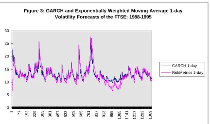
(10) Risk Management and Analysis: Measuring and Modelling Financial Risk. 10. (C. Alexander, Ed) Wileys, (1998). coefficient is 0.94 for all markets, and the reaction coefficient is 0.06 for all markets. But if one estimates these coefficients rather than imposes them, it appears that λ=0.94 is too high for most markets. For example, in the FTSE series shown in figure 3, the GARCH persistence coefficient is 0.88, and so the GARCH volatility series dies out more quickly than the RiskMetrics. However their reaction coefficient is the same (0.06) and so both volatilities exhibit a similar size of market reaction in figure 3.. Figure 3: GARCH and Exponentially Weighted Moving Average 1-day Volatility Forecasts of the FTSE: 1988-1995 30 25 20 GARCH 1-day. 15. RiskMetrics 1-day. 10 5. 1369. 1293. 1217. 1141. 1065. 989. 913. 837. 761. 685. 609. 533. 457. 381. 305. 229. 153. 77. 1. 0. The RiskMetrics daily data do have some other problems, which are explained in Alexander, 1996, but these are not insurmountable.9 However, the RiskMetrics forecasts of volatility over the next month behave in a rather strange fashion. Since the EWMA methodology is only really applicable to one-step-ahead forecasting the correct thing would be to smooth 25-day returns, but. 9. In fact all the RiskMetrics matrices have low rank - either because EWMA use insufficient data for the size of matrix, or because of the linear interpolation of yield curve data..

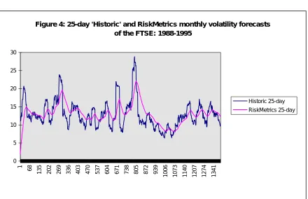
(11) Risk Management and Analysis: Measuring and Modelling Financial Risk. 11. (C. Alexander, Ed) Wileys, (1998). there is not enough data. Instead, JP Morgan have applied exponential smoothing with a value of λ=0.97 to the 25-day equally weighted variance. But this series will be full of 25-day ‘ghost features’ (see figure 1) so the exponential smoothing has the effect of augmenting the very ‘ghost features’ which they seek to diminish. After a major market movement the equally weighted 25day series jumps up immediately - as would any sensible volatility forecast. But the RiskMetrics™ monthly data hardly reacts at all, at first, then it gradually increases over the next 25 days to reach a maximum exactly 25 days after the event. The proof of this is simple: denote by st2 the 25-day 'historic' variance series, so the monthly variance forecast is σ$ 2t σ$ 2t > σ$ 2t −1. ⇔. =. (1 − λ ) st2−1 + λ σ$ 2t −1 . Clearly. st2−1 > σ$ t2−1 . At the 'ghost feature' st2 drops dramatically, and so the maximum. value of σ$ 2t will occur at this point.. Figure 4: 25-day 'Historic' and RiskMetrics monthly volatility forecasts of the FTSE: 1988-1995 30 25 20 Historic 25-day 15. RiskMetrics 25-day. 10 5. 1341. 1274. 1207. 1140. 1073. 1006. 939. 872. 805. 738. 671. 604. 537. 470. 403. 336. 269. 202. 135. 1. 68. 0. Figure 4 compares the RiskMetrics monthly forecasts for the FTSE with the equally weighted 25day ‘historic’ forecasts, during the same period as in figure 3. Neither forecast is useful: the ‘historic’ forecast peaks at the right time, the day after a significant maret movement, but it stays high for 25-days, when it should probably be declining. The RiskMetrics 25-day forecast hardly.

(12) Risk Management and Analysis: Measuring and Modelling Financial Risk. 12. (C. Alexander, Ed) Wileys, (1998). reacts at all to a market movement, but it slowly increases during the next 25-days so that the largest forecast of the volatility over the next month occurs 25-days too late. 4.2.3 Volatility Term Structures in Moving Average Models: The Square Root of Time Rule Term structure volatility forecasts which are consistent with moving average models are constant, because that is the underlying assumption on volatility. Moving average models are, after all, estimation methods, not forecasting methods. We can of course say that our current estimate of volatility is to be taken as all future forecasts, and this is what is generally done. The current oneday volatility estimate is taken to be the one-day forward volatility forecast at every point in the future. Term structure forecasts - forecasts of the volatility of h-day returns for every maturity h - are then based on the ‘square root of time’ rule. This rule simply calculates h-day standard deviations as √h times the daily standard deviation. It is based on the assumption that daily log returns are independently and identically distributed, so the variance of h-day returns is just h times the variance of daily returns. But since volatility is just an annualised form of the standard deviation, and since the annualising factor is - assuming 250 days per year - √250 for daily returns but √(250/h) for h-day returns, the square root of time rule is equivalent to the Black-Scholes assumption that current levels of volatility remain the same. The square root of time rule implies the assumption of constant volatility. This follows from the assumption that log returns are independent and identically distributed. To see this, introduce the notation rt,h for an h-day return at time t, and so approximately rt,h = ln(Pt+h) - ln(Pt) where Pt denotes the price at time t. Clearly rt,h = rt,1 + rt+1,1+……+ rt+h-1,1.

(13) Risk Management and Analysis: Measuring and Modelling Financial Risk. 13. (C. Alexander, Ed) Wileys, (1998). and if we assume that 1-day returns are independent and identically distributed with constant variance σ2 we have V(rt,h) = hσ2. Annualising this into a volatility requires the use of an annualising factor 250/h, being the number of h-periods per year: h-period vol = 100 √(250/h) √V(rh,t) = 100 √(250/h) √(hσ2) = 100 √(250σ2) = 1-period vol That is, volatility term structures are constant. Constant term structures are a limitation of exponentially weighted moving average methods. The reason for this is that financial volatility tends to come in ‘clusters’, where tranquil periods of small returns are interspersed with volatile periods of large returns10. Thus volatility term structures should mean-revert, with short term volatility lying either above or below the long term mean depending on whether current conditions are high or low volatility. Clearly moving averages are quite limited in this respect. Substantial mispricing of volatility can result from these methods, as a number of large banks have recently discovered.. 4.3 GARCH Models in Finance 4.3.1 Introduction The unfortunate acronym 'GARCH' is nevertheless essential, since it stands for generalised autoregressive conditional heteroscedasticity! Heteroscedasticity means 'changing variance', so conditional heteroscedasticity means changing conditional variance. A time series displays conditional heteroscedasticity if it has highly volatile periods interspersed with tranquil periods: i.e. there are 'bursts' or 'clusters' of volatility. Autoregressive means 'regression on itself', and this refers to the method used to model conditional heteroscedasticity in GARCH models. Most financial time series display autoregressive conditional heteroscedasticity. A typical example of conditionally heteroscedastic returns in high frequency data - minute by minute data on cotton. 10. As long ago as 1963 Benoit Mandlebrot observed that financial returns time series exhibit periods of volatility interspersed with tranquillity, where ‘Large returns follow large returns, of either sign.....’.

(14) Risk Management and Analysis: Measuring and Modelling Financial Risk. 14. (C. Alexander, Ed) Wileys, (1998). futures - is shown in figure 5. Note that two types of news events are apparent. The first volatility cluster shows an anticipated announcement, which turned out to be good news: the market was increasingly turbulent before the announcement, but the large positive return at that time shows that punters were pleased, and the volatility soon decreased. The later cluster of volatility shows increased turbulence following an unanticipated piece of bad news - the large negative return what is often referred to as the ‘leverage’ effect (see section 4.3.2 (iv)) NOTE TO COPY EDITOR <Figure 5 here - same as figure 8.4 from 1st edition, and formatted with caption and frame as in the previous figures please> At the root of understanding GARCH is the distinction between conditional (stochastic) and unconditional (constant) volatility. These ideas are based on different stochastic processes which are assumed to govern the returns data. Figure 6 illustrates the difference between conditional and unconditional distributions of returns. In figure 6(a) the stochastic process which generates the time series data on returns is assumed to be independent and identically distributed. This same distribution governs each of the data points, and since they are independent we may as well redraw the data without taking account of the dynamic ordering, along a line. The data are then considered to be random draws from a single distribution, called the unconditional distribution (figure 6(b)). However, in figure 6(c) the same data are assumed to be generated by a stochastic process with time varying volatility. In this case it is not realistic to collapse the data into a single distribution, ignoring the dynamic ordering. The conditional distribution changes at each point in time, and in particular the volatility process is stochastic. NOTE TO COPY EDITOR <Figure 6 here please, please have the hand drawn figure attached properly set by printer>. The first ARCH model, introduced by Rob Engle (1992) was later generalised by Tim Bollerslev (1986), and many variations on the basic ‘vanilla’ GARCH model have been introduced in the last.

(15) Risk Management and Analysis: Measuring and Modelling Financial Risk. 15. (C. Alexander, Ed) Wileys, (1998). ten years.11 The idea of GARCH is to add a second equation to the standard regression model an equation which models the conditional variance. The first equation in the GARCH model is the conditional mean equation.12 This can be anything, but because the focus of GARCH is on the conditional variance equation13 it is usual to have a very simple conditional mean equation, such as rt = constant + εt. Note that the dependent variable (the input to the GARCH model) is always the returns series, and in the simple case that rt = constant + εt the unexpected return εt is just the mean deviation return, because the constant will be the average of returns over the data period. Of course we can put whatever explanatory variables we want in the conditional mean equation of a GARCH model, but should err on the side of parsimony if we want the model estimation procedure to converge properly (see section 4.3.4). The conditional mean equation rt = constant + εt is fairly standard. A GARCH model conditional variance equation provides an easy analytic form for the stochastic volatility process in financial returns. GARCH models differ only because the conditional variance equations are specified in different forms, or because of different assumptions about the conditional distribution of unexpected returns. In normal GARCH models we assume that εt is conditionally normally distributed with 2 conditional variance σ t . The unconditional returns distributions will then be leptokurtic - that is,. have fatter tails than the normal - because the changing conditional variance allows for more outliers or unusually large observations. However in high frequency data there may still be insufficient leptokurtosis in normal GARCH to capture the full extent of kurtosis in the data, and. 11. For excellent reviews of the enormous literature on GARCH models in finance see Bollerslev et.al. (1992) and (1993). 12 The unconditional mean of a stationary time series y is a single number, a constant. It is denoted E(y) or µ, and is usually estimated very simply by the sample mean. On the other hand, the conditional mean varies over time, and is commonly measured by a linear regression model. The conditional mean is denoted Et(yt) or µt or E(ytΩt), where Ωt is the information set available at time t (so Ωt includes yt-1 and any other values which are known at time t). 13 The unconditional variance of a stationary time series y is a constant, denoted V(y) or σ2. It is often estimated by a moving average, as explained in the previous section. On the other hand, the conditional variance σt 2 is often denoted Vt(yt) or Vt(ytΩt). Like the conditional mean, its’ estimates will form a time-varying series..

(16) Risk Management and Analysis: Measuring and Modelling Financial Risk. 16. (C. Alexander, Ed) Wileys, (1998). in this case a t-distribution could be assumed (Baillie and Bollerslev, 1989, 1990), or a GARCH model defined on a mixture of normals (see section 4.6). Square rooting the GARCH conditional variance series, and expressing it as an annualised percentage in the usual way yields a time-varying volatility estimate. But unlike the moving average methods just described, the current estimate is not taken to be the forecast of volatility over all future time horizons. Instead, by first estimating the GARCH model parameters, we can then construct mean-reverting forecasts of volatility as explained in section 4.3.3. GARCH is sufficiently flexible that these forecasts can be adapted to any time period. For example, when valuing Asian options, volatility options, or measuring risk capital requirements it is often necessary to forecast forward volatility, such as a 1-month volatility but in 6 months time. This flexibility is one of the many advantages of GARCH modelling over the moving average methods just described. Very many different types of GARCH models have been proposed in the academic literature, but only a few of these have found good practical applications. The bibliography contains only a fraction of the most useful empirical research papers on GARCH. In the next section we review some of the univariate models which have received the most attention: ARCH, GARCH, IGARCH, AGARCH, EGARCH, Components GARCH and Factor ARCH. There is little doubt that these GARCH volatility models are easy and attractive to use. A summary of their useful applications in financial risk management is given in section 4.5. However, in a climate where firm-wide risk management is the key, there is a pressing need to model volatilities and correlations in the context of large covariance matrices which cover all the risk factors relevant to the operations of a firm. Unfortunately it is not easy to use GARCH for large systems. In the last part of section 3 we look at the problems with direct estimation of high dimensional multivariate GARCH models and propose a new method for generating large GARCH covariance matrices. 4.3.2 A Survey of GARCH Volatility Models 1. ARCH.

(17) Risk Management and Analysis: Measuring and Modelling Financial Risk. 17. (C. Alexander, Ed) Wileys, (1998). The original model of autoregressive conditional heteroscedasticity introduced in Engle (1982) has the conditional variance equation σ t2. = α0 + α1 εt2−1 α 0 > 0,. + ... + α p ε t2− p. (9). α1 , ...., α p ≥ 0. where the constraints on the coefficients are necessary to ensure that the conditional variance is always positive. This is the ARCH(p) conditional variance specification, with a memory of p time periods. This model captures the conditional heteroscedasticity of financial returns by using a moving average of past squared unexpected returns: If a major market movement in either direction occurred m periods ago (m ≤ p) the effect will be to increase today's conditional variance. This means that we are more likely to have a large market move today, so 'large movements tend to follow large movements ... of either sign'. 2. VANILLA GARCH The generalisation of Engle's ARCH(p) model by Bollerslev (1986, 1987) adds q autoregressive terms to the moving averages of squared unexpected returns: it takes the form σ t2 = ω + α1ε t2−1 +...+ α p ε t2− p + β1σ t2−1 +...+ βq σ t2− q. (10). ω > 0, α1 ,..., α p , β1 , ..., βq ≥ 0. The parsimonious GARCH(1,1) model, which has just one lagged error square and one autoregressive term, is most commonly used: σ t2 = ω + α εt2−1 + β σ t2−1 ω > 0, α β ≥ 0. (11). It is equivalent to an infinite ARCH model, with exponentially declining weights on the past squared errors:.

(18) Risk Management and Analysis: Measuring and Modelling Financial Risk (C. Alexander, Ed) Wileys, (1998). σ t2 = ω + α ε t2− 1 + β σ t2− 1 = ω + α ε t2− 1 + β ( ω + α ε t2− 2 + β ( ω + α ε t2− 3 + β (..... = ω / (1 − β ) + α ( ε t2− 1 + β ε t2− 2 + β 2 ε t2− 3 + ....). The above assumes that the GARCH(1,1) lag coefficient β is less than 1. In fact a few calculations show that the unconditional variance corresponding to a GARCH(1,1) conditional variance is σ2. = ω / (1 − α − β ). (12). and so not only must the GARCH return coefficient α also be less than 1, the sum α + β ≤ 1. In financial markets it is common to find GARCH lag coefficients in excess of 0.7 but GARCH returns coefficients tend to be smaller, usually less than 0.25. The size of these parameters determine the shape of the resulting volatility time series: large GARCH lag coefficients indicate that shocks to conditional variance take a long time to die out, so volatility is ‘persistent’; large GARCH reurns coefficients mean that volatility is quick to re-act to market movements, and volatilities tend to be more 'spiky'. Figure 7 shows US dollar rate GARCH(1,1) volatilities for Sterling and the Japanese Yen. Cable volatility is more persistent (its lag coefficient is 0.931 compared with 0.839 for the Yen/$) - the Yen/$ is more spiky (its return coefficient is 0.094 compared with 0.052 for Cable).14 See Alexander (1995a) for more details. NOTE TO COPY EDITOR <Figure 7 here - same as figure 8.6 of 1st edition but please reduce size and line thickness in charts> The constant ω determines the long-term average level of volatility to which GARCH forecasts converge (see section 4.3.3). Unlike the lag and return coefficients, its value is quite sensitive to. 14. These are slightly different from the values given in table 1 below, because firstly they use daily data (table 1 exchange rates are based on weekly data) and secondly a different data estimation period is used.. 18.

(19) 19. Risk Management and Analysis: Measuring and Modelling Financial Risk (C. Alexander, Ed) Wileys, (1998). the length of data period used to estimate the model.15 If a period of many years is used, during which there were extreme market movements, the estimate of ω will be high. So current volatility term structures will converge to a higher level. Consider for example, the generation of a GARCH volatility term structure on the FTSE today. Long term average volatility levels in the FTSE are around 13%, but if we include the Black Monday period in the data used to estimate today’s GARCH model, we would find current long term volatility forecasts at around 15%. 3. INTEGRATED GARCH When α + β = 1 we can put β = λ and re-write the GARCH(1,1) model as σ t2 = ω + (1 − λ ) ε t2−1 + λ σ t2−1. 0≤ λ ≤1. (13). Note that the unconditional variance (12) is now undefined - indeed we have a non-stationary GARCH model called the Integrated GARCH (I-GARCH) model, for which term structure forecasts do not converge. Our main interest in the I-GARCH model is that when ω = 0 it is equivalent to an infinite EWMA, such as those used by RiskMetrics. This may be seen by repeated substitution in (13): σ t2 = ω + (1 − λ ) εt2−1 + λ (ω + (1 − λ ) εt2− 2 + λ (ω + (1 − λ ) εt2− 3 + λ (.... = ω / (1 − λ ) + (1 − λ )(εt2−1 + λ εt2−2 + λ2 εt2− 3 +.....). (14). Currency markets commonly have close to integrated GARCH models, and this has prompted major players such as Salomon Bros. to formulate new models for currency GARCH, such as the components GARCH model described below (see Chew, 1993). 4. ASYMMETRIC GARCH The asymmetric GARCH (A-GARCH) model (Engle and Ng, 1993) has conditional variance equation. For this reason it is common to impose a value of ω = (1 - α − β) σ2 from equation (12), using an unconditional volatility estimate for σ2. 15.

(20) 20. Risk Management and Analysis: Measuring and Modelling Financial Risk (C. Alexander, Ed) Wileys, (1998). σ t2. = ω + α (εt −1 − ξ ) 2 + β σ t2−1. ω > 0,. α, β,ξ ≥ 0. (15). In this model, negative shocks to returns (εt-1 < 0) induce larger conditional variances than positive shocks. Thus the A-GARCH model is appropriate when we expect more volatility following a market fall than following a market rise. This ‘leverage effect’ is a common feature of financial markets, particularly equities. 5. EXPONENTIAL GARCH The non-negativity constraints of the GARCH models considered so far can unduly restrain the dynamics of conditional variances so obtained. Nelson (1991) eliminated the need for such constraints in his exponential GARCH model by formulating the conditional variance equation in logarithmic terms log σ t2 = α + g ( z t −1 ) + β log σ t2−1. (16). where zt = εt /σt , so zt is standard normal, and  2 . g( z t ) = ω z t + λ  z t − π . (17). The asymmetric response function g(.) , which is illustrated in figure 8, provides the leverage effect just as in the AGARCH model. Many studies have found that the E-GARCH model fits financial data very well (for example, see Taylor, 1994, Heynen et. al., 1994, and Lumsdaine, 1995) but it is much more difficult to obtain volatility forecasts using this model. NOTE TO COPY EDITOR <Figure 8 here - same as figure 8.7 from 1st edition> 6. COMPONENTS GARCH.

(21) Risk Management and Analysis: Measuring and Modelling Financial Risk. 21. (C. Alexander, Ed) Wileys, (1998). In practice, estimation of a GARCH model over a rolling data window will generate a term structure of volatility forecasts for each day. In each of these term structures, as volatility maturity increases, GARCH forecasts should converge to a long-term level of volatility (see section 4.3.3). As the data window is rolled different long-term levels will be estimated, corresponding to different estimates of the GARCH parameters. The components model extends this idea of timevarying 'baseline' volatility to allow variation within the estimation period (Engle and Lee, 1993 and Engle and Mezrich, 1995). To understand the components model, note that when α + β < 1 the GARCH(1,1) conditional variance is often estimated by imposing ω. The model may be written in the form. σ t2 = (1 − α − β )σ 2 + α εt2−1 + β1σ t2−1. (18). = σ 2 + α (εt2−1 − σ 2 ) + β (σ t2−1 − σ 2 ). where σ2 is defined by (12). We now replace σ2 by a time-varying permanent component in conditional variance: q t = ω + ρ (q t −1 − ω ) + φ (εt2−1 − σ t2−1 ). (19). and then the formulation (18) becomes σ t2 = q t + α (εt2−1 − q t −1 ) + β (σ t2−1 − q t −1 ). (20). The equations (19) and (20) together define the components model. If ρ = 1, the permanent component - to which long-term forecasts mean revert - is just a random walk. 7. FACTOR GARCH Factor GARCH allows individual volatilities and correlations to be estimated and forecast from a single GARCH volatility - the volatility of the market. Consider the simple capital asset pricing.

(22) Risk Management and Analysis: Measuring and Modelling Financial Risk. 22. (C. Alexander, Ed) Wileys, (1998). model, where individual asset or portfolio returns are related to market returns Mt by the regression equation rit = αi + βi M t + εit. i = 1,2,....., n. (21). Denoting by σit the standard deviation of asset i at time t and by σijt the covariance between assets i and j at time t, equation (21) yields σ it2. =. 2 βi 2 σ Mt. σ ijt2. 2 = βi β j σ Mt. + σ ε2it + σ εit ε jt. (22). From a simultaneous estimation of the n linear regression equations in (22) we can obtain estimates of the factor sensitivities βi and the error variances and covariances. These, and the univariate GARCH estimates of the market volatility σM are then used to generate individual asset volatilities and correlations using (22). The idea is easily extended to a model with more than one risk factor, see Engle, Ng and Rothschild (1990).. 4.3.3 GARCH Volatility Term Structure Forecasts One of the beauties of GARCH is that volatility and correlation forecasts for any horizon can be constructed from the one estimated model. First we use the estimated GARCH model to give us forecasts of instantaneous forward volatilities, that is the volatility of rt+j, made at time t and for every step ahead j. The instantaneous GARCH forecasts are calculated analytically: for example, in the GARCH(1,1) model σ$t2+1 = ω$ + α$ εt2 + β$ σ$t2 and the j-step ahead forecasts are computed iteratively16 as. 16. We only know the unexpected return at time t, not εt+j for j>0. But E(εt+j2) = σt+j2.. (23).

(23) Risk Management and Analysis: Measuring and Modelling Financial Risk. 23. (C. Alexander, Ed) Wileys, (1998). σ$t2+ j = ω$ + (α$ + β$ ) σ$t2+ j −1. (24). To get a term structure of volatility forecasts from these forward volatilities note that the (logarithmic) return at time t over the next n periods is. rt ,n. =. n. ∑r. t+ j. j =1. The volatility term structure is a plot of the volatility of these returns for n=1,2,3,……. Since Vt (rt ,n ) =. n. ∑V (r i =1. t. t +i. ) +. ∑ ∑ COV (r t. i. t +i. , rt + j ). (25). j. the GARCH forecast of n-period variance is the sum of the instantaneous GARCH forecast variances, plus the double sum of the forecast autocovariances between returns. This double sum will be very small compared to the first sum on the right hand side of (25), indeed in the majority of cases the conditional mean equation in a GARCH model is simply a constant, so returns are independent and the double sum is zero.17 Hence we ignore the autocovariance term in (25) and construct n-period volatility forecasts simply by adding the j-step-ahead GARCH variance forecasts (and then square-rooting and annualising in the usual way).18. Even in an AR(1)-GARCH(1,1) model (with autocorrelation coefficient ρ in the conditional mean equation) (25) becomes 17. σ$t2,n =. n. ∑ σ$ i =1. 2 t +i. + σ$t2 [ ρ (1 − ρ n ) / (1 − ρ )]2. and the first term clearly dominates the second. 18 In this way we can also construct any sort of forward volatility forecasts, such as 3-month volatility but for a period starting six months from now..

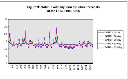
(24) Risk Management and Analysis: Measuring and Modelling Financial Risk. 24. (C. Alexander, Ed) Wileys, (1998). Figure 9: GARCH volatility term structure forecasts of the FTSE: 1988-1995 30 25 GARCH 1-day. 20. GARCH 10-day GARCH 30-day. 15. GARCH 60-day GARCH 120-day. 10 5. 1341. 1274. 1207. 1140. 1073. 939. 1006. 872. 805. 738. 671. 604. 537. 470. 403. 336. 269. 202. 135. 1. 68. 0. Figure 9 shows 1-day, 10-day 30-day 60-day and 120-day volatility forecasts for the FTSE from 1988-1995. Note how the forecasts of different maturities converge to the long-term volatility level of around 13%. During a volatile period GARCH term structures converge to this level from above (figure 10(a)) and during a tranquil period they converge from below (figure 10(b)) ..

(25) Risk Management and Analysis: Measuring and Modelling Financial Risk (C. Alexander, Ed) Wileys, (1998). Figure 10(a): GARCH volatility term structures of US Dollar rates on April 13 1995 16. Volatility Forecast. 14 12 10 8. GBP. 6. DEM JPY. 4 2 191. 181. 171. 161. 151. 141. 131. 121. 111. 91. 101. 81. 71. 61. 51. 41. 31. 21. 1. 11. 0 Days. Figure 10(b): GARCH volatility term structures of US Dollar rates on March 2 1995 12. Volatility Forecast. 10 8. GBP DEM. 6. JPY 4 2. 199. 188. 177. 166. 155. 144. 133. 122. 111. 100. 89. 78. 67. 56. 45. 34. 23. 12. 1. 0 Days. The speed of convergence in GARCH(1,1) depends on α + β. Currency markets generally have the highest values of α + β, and hence the slowest convergence. The speed of convergence in equity and commodity GARCH models tends to be faster, and bond markets often have the. 25.

(26) Risk Management and Analysis: Measuring and Modelling Financial Risk. 26. (C. Alexander, Ed) Wileys, (1998). lowest α + β and the fastest converge of volatility term structures to the long-term level (see section 4.3.4). 4.3.4 Estimating GARCH Models: Methods and Results. Most of the models described above are available as pre-programmed procedures in econometric packages such as S-PLUS, TSP, EVIEWS and MICROFIT, and in GAUSS and RATS, GARCH procedures can be written, as explained in the manuals. The method used to estimate GARCH model parameters is maximum likelihood estimation, which is a powerful and general statistical procedure, widely used because it always produces consistent estimates.. The idea is to choose parameter estimates to maximise the likelihood of the data under an assumption about the shape of the distribution of the data generation process. For example, if we assume a normal data generation process with mean µ and variance σ2 then the likelihood of getting returns r1 , r2 , ...., rT is. L ( µ , σ |r1 , r2 , .... , rT ) 2. where. f (r ) =. 1 2πσ 2. =. 1 exp{− 2. T. ∏ f (r ) t =1. t.  r − µ   }  σ . (26). 2. (27). Choosing µ and σ2 to maximise L (or equivalently to minimise -2logL) yields the maximum likelihood estimates of these parameters.. In GARCH models there are more than just two parameters to estimate, and the likelihood functions are more complex (for example, see Engle, 1982 and Bollerslev, 1986) but the principle is the same. Problems arise though, because the more parameters in the likelihood function the 'flatter' it becomes, and therefore more difficult to estimate. For this reason the GARCH(1,1) model is preferred to an ARCH model with a long lag, and parameterizations of conditional mean.

(27) Risk Management and Analysis: Measuring and Modelling Financial Risk. 27. (C. Alexander, Ed) Wileys, (1998). equations are as parsimonious as possible - often we use just a single constant in the conditional mean.. Convergence problems with GARCH models can arise because gradient search algorithms used to maximize the likelihood functions fall off a boundary. Sometimes this problem can be mitigated by changing the starting values of the parameters, or knocking a few data points off the beginning of the data set so the likelihood function has a different gradient at the beginning of the search. The time taken for GARCH models to converge will be greatly increased unless analytic derivatives are used to calculate the gradient in the search. For leptokurtic data, t-distributed GARCH models have lost ground in favour of normal mixture GARCH models since they require numerical derivatives to be calculated at each iteration.. However, most univariate GARCH models should encounter few convergence or robustness problems if they are well-specified. Care should be taken over the re-specification of initial conditions if the coefficients estimates hit a boundary value, and sometimes minor changes in the returns data can induce the occasional odd value of coefficients. These will be evident in rolling GARCH models, where convergence conditions may need re-setting. In some cases the coefficient values take some time to settle down but once the model is properly tuned to the data it can be updated daily or weekly with few problems..

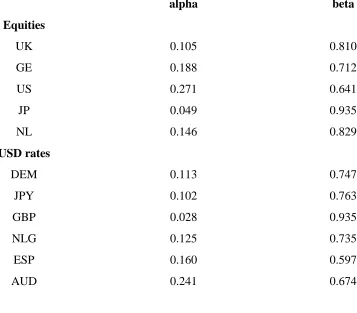
(28) Risk Management and Analysis: Measuring and Modelling Financial Risk. 28. (C. Alexander, Ed) Wileys, (1998) Table 1: Approximate GARCH(1,1) parameters for equity markets and USD exchange rates. alpha. beta. UK. 0.105. 0.810. GE. 0.188. 0.712. US. 0.271. 0.641. JP. 0.049. 0.935. NL. 0.146. 0.829. DEM. 0.113. 0.747. JPY. 0.102. 0.763. GBP. 0.028. 0.935. NLG. 0.125. 0.735. ESP. 0.160. 0.597. AUD. 0.241. 0.674. Equities. USD rates. Table 1 gives an idea of what to expect when estimating GARCH(1,1) parameters in some of the major currency and equity markets. Note that very few of these markets have persistence parameters which are as large as the value 0.94 used for the RiskMetrics data. Of course the GARCH parameters depend on the data frequency and estimation period, but they should be fairly robust to these differences. When rolling the estimation of a GARCH model day by day, significant changes in the parameters should occur consequent to major market movements only. Bond market GARCH models are more difficult to estimate, particularly since some maturities can be quite illiquid. To estimate and forecast volatilities and correlations for an entire yield curve, the orthogonal GARCH model is highly recommended (see section 4.3.7).. 4.3.5 Choosing the Data Period and the Appropriate GARCH Model.

(29) Risk Management and Analysis: Measuring and Modelling Financial Risk. 29. (C. Alexander, Ed) Wileys, (1998). The plain ‘vanilla’ GARCH(1,1) model - even without asymmetric or leptokurtic effects - already offers many advantages over the moving average methods described in section 4.2, and many financial institutions are currently basing their systems on this model. One of the questions that senior management will want to address is whether such a simple GARCH model does the trick is it capturing the right type of volatility clustering in the market - or should we be using some sort of complex fractionally integrated GARCH model like the house next door? In this section we show how to diagnose whether you have a good GARCH model or not, and how to employ data to the best advantage.. A test for the presence of ARCH effects in returns is obtained by looking at the autocorrelation in the time series of squared returns . Standard autocorrelation test statistics may be used, such as the Box-Pierce Q ∼ χ2 (p) :. Q = T. p. ∑ ϕ( n ). 2. (28). n =1. where ϕ(n) is the nth order autocorrelation coefficient in squared returns T. ϕ( n ) =. ∑r. t = n +1 T. 2. rt 2− n. t. ∑r t =1. (29) 4. t. One of the main specification diagnostics in GARCH models is to first standardise the returns by dividing by the estimated GARCH standard deviation, and then test for autocorrelation in squared standardised returns. If it has been removed, the GARCH model is doing its job. But what if several GARCH models account equally well for GARCH effects? In that case choose the GARCH model which gives the highest likelihood, either in-sample or in post-sample predictive tests.. The two important considerations in choosing data for GARCH modelling are the data frequency and the data period. It is usual to employ daily or even intra-day data rather than weekly data.

(30) Risk Management and Analysis: Measuring and Modelling Financial Risk. 30. (C. Alexander, Ed) Wileys, (1998). since convergence problems could be encountered on low frequency data due to insufficient ARCH effects. If tic data are used the time bucket should be sufficiently large to ensure there are no long periods of no trades, and by the same token bank holidays may cause problems so it is often better to deviate from the standard time-series practise of using equally spaced daily data, and not fill in the zero returns caused by back holidays.. When it comes to choosing the amount of historical data for estimating GARCH models, the real issue is whether you want major market events from several years ago to influence your forecasts today. As we have already seen, including Black Monday in equity GARCH models has the effect of raising long-term volatility forecasts by several percent. In the orthogonal GARCH model of section 4.3.7 it is also important not to take too long a data period, since the principal components are only unconditionally orthogonal so the model will become ill-conditioned if too long a data period is chosen.19 On the other hand, a certain amount of data is necessary for the likelihood fuction to be sufficiently well defined. Usually at least one or two years of daily data are necessary to ensure proper convergence of the model.. 4.3.6 Multivariate GARCH. Univariate GARCH models commonly converge in an instant, the only real problems being lack of proper specification by the user, or inappropriate data. But there are very serious computational problems when attempting to build large positive definite GARCH covariance matrices which are necessary if one is to net the risks from all positions in a large trading book.. This section reviews the basic multivariate GARCH models, discussing the inevitable computational problems if one attempts direct estimation of full GARCH models in large dimensional systems. The unconditional variance of a multivariate process is a positive definite. For risk management purposes, currently one does not need to go further back than 1st January 1993. The major disruptions to financial markets during 1992 are best left out of ordinary everyday volatilities, but can easily be recreated when the model is being stressed.. 19.

(31) Risk Management and Analysis: Measuring and Modelling Financial Risk. 31. (C. Alexander, Ed) Wileys, (1998). matrix, the covariance matrix, already defined in the introduction. The conditional variance of a multivariate process is a time-series of matrices, one matrix for each point in time. It is not surprising therefore that estimation of these models can pose problems! The convergence problems outlined in section 4.3.4 can become insurmountable even in relatively low dimensional systems, so parameterizations of multivariate GARCH models should be as parsimonious as possible. There are many ways that multivariate GARCH can be constrained in order to facilitate their estimation but these methods often fall down on at least one of two counts: either they are only applicable to systems of limited dimension (something like 5-10 factors being the maximum) or they need to make unrealistic assumptions on parameters that are not confirmed by the data (see Engle and Kroner, 1995). However, section 4.3.7 presents a new method which falls down on neither count. It uses orthogonal approximations to generating arbitrary large GARCH covariance matrices using only univariate GARCH models.. Consider first the bivariate GARCH model, appropriate only if we are just interested in the correlation between two returns series, r1 and r2 . There will now be two conditional mean equations, which can be anything we like but for the sake of parsimony we shall assume that each equation gives the return as a constant plus error: r1,t = ϕ11 + ε1,t r2 ,t = ϕ 21 + ε2 ,t. In a bivariate GARCH there are three conditional variance equations, one for each conditional variance and one for the conditional covariance. Since all parameters will be estimated simultaneously the likelihood can get very flat indeed, so we need to use as few parameters as possible. In this section we introduce the two standard parameterizations of multivariate GARCH models: the vech and the BEKK.. In the vech parameterization each equation is a GARCH(1,1):.

(32) 32. Risk Management and Analysis: Measuring and Modelling Financial Risk (C. Alexander, Ed) Wileys, (1998). σ 12,t = ω1 + α1ε12,t −1 + β1σ 12,t −1 σ 22,t = ω 2 + α2 ε22,t −1 + β2 σ 22,t −1. (30). σ 12 ,t = ω + α3 ε1,t −1ε2 ,t −1 + β3σ 12 ,t −1 As usual, constraints on the coefficients in (30) are necessary to ensure positive definiteness of the covariance matrices. To obtain time-series of GARCH correlations we simply divide the estimated covariance by the product of the estimated standard deviations, at every point in time (see figure 11). <Figure 11 here - same as fig 8.8 from 1st edition>. When considering systems with more than two returns series we need matrix notation. The matrix form of equations (30) is. vech (Ht ). =. A. +. B vech (ξt-1ξt-1' ). +. C vech (Ht-1). (31). where Ht is the conditional variance matrix at time t. So vech(Ht) = (σ1t2 , σ2t2 , σ12t )' , and ξt = ( ε1t, ε2t)' , A = (ω1, ω2, ω3)', B = diag( α1, α2, α3) and C = diag (β1, β2, β3) , with the obvious generalisation to higher dimensions.. There are severe cross equation restrictions in the vech model, for example the conditional variances are not allowed to affect the covariances and vice-versa. In some markets these restrictions can lead to substantial differences between the vech and BEKK estimates so the vech model should be employed with caution.. A more general formulation, which involves the minimum number of parameters whilst imposing no cross equation restrictions and ensuring positive definiteness for any parameter values is the BEKK model (after Baba, Engle, Kraft and Kroner who wrote the preliminary version of Engle and Kroner, 1995). This parameterization is given by.

(33) Risk Management and Analysis: Measuring and Modelling Financial Risk. 33. (C. Alexander, Ed) Wileys, (1998). Ht. =. A'A. +. B' ξt-1ξt-1' B. +. C' Ht-1 C. (32). where A, B and C are general nxn matrices (A is triangular). The BEKK parameterization for a bivariate model involves eleven parameters, only two more than the vech. But for higher dimensional systems the extra number of parameters increases, and completely free estimation becomes very difficult indeed. Often it is necessary to let B and C be scalar matrices, to reduce the number of parameters needing estimation and so improve the likelihood surface and, hopefully, achieve convergence. More details are given in Bollerslev et. al. (1992) and Bollerslev et. al. (1994) .. A useful technique for calibrating multivariate GARCH is to compare the multivariate volatility estimates with those obtained from direct univariate GARCH estimation. The multivariate GARCH volatility term structure forecasts are computed as outlined in section 4.3.4. and correlation forecasts are calculated in a similar fashion: simply by iterating conditional covariance forecasts and summing these to get n-period covariance forecasts.20 These are then divided by the product of n-period volatility forecasts for correlation term structures: ρ$t ,n. = σ$12 ,t ,n /σ$1,t ,n σ$2 ,t ,n. 4.3.7 Generating Large GARCH Covariance Matrices: Orthogonal GARCH. The computations required to estimate very large GARCH covariance matrices by direct methods are simply not feasible at the present time. However indirect ‘orthogonalization’ methods can be used to produce the large covariance matrices necessary to measure risk in large portfolios. This.

(34) Risk Management and Analysis: Measuring and Modelling Financial Risk. 34. (C. Alexander, Ed) Wileys, (1998). method is introduced, explained and verified for all major equity, currency and fixed income markets by Alexander and Chibumba (1997).. In orthogonal GARCH the risk factors from all positions across the entire firm are first divided into reasonably highly correlated categories, according to geographic locations and instrument types. Principal components analysis is then used to orthogonalize each sub-system of risk factors, univariate GARCH is applied to the principal components to obtain the (diagonal) covariance matrix, and then the factor weights from the principal components analysis are used to ‘splice’ together the large covariance matrix for the whole enterprise.. An example explaining the method for just two risk factor categories can easily be extrapolated to any number of risk factor categories: Suppose P = (P1 , ... Pn ) are the principal components of the first system (n risk factors) and let Q = (Q1 ,...Qm ) be the principal components of the second system (m risk factors).21 Denote by A (nxn) and B (mxm) the factor weights matrices of the first and second systems. Within factor covariances are given by AV(P)A’ and BV(Q)B’ respectively and cross factor covariances are ACB’ where C denotes the mxn matrix of covariances of principal components.. An illustration of this method applies to a system of equity indices and USD exchange rates (Alexander and Chibumba, 1997). The system is just small enough to compare the ‘splicing’ method with full multivariate GARCH estimation and figure 12 shows one of the resulting. 20. To see this, note that COVt ( r1,t ,n , r2 ,t ,n ). covariances gives σ$12 ,t ,n = 21. =. n. ∑ COV (r. i , j =1. t. 1,t + i. , r2 ,t + j ) . Ignoring non-contemporaneous. n. ∑ σ$ i =1. 12 ,t + i. .. One of the advantages of principal components analysis is to reduce dimension, and this is certainly an attractive proposition for the yield curve (see chapter ?), or for systems when the reduction in ‘noise’ obtained by using only a few principal components makes correlations more stable. However it is the orthogonality property of principal components which is the primary attraction here, and if one does not retain the full number of principal components, we cannot ensure positive definiteness of the final covariance matrix..

(35) Risk Management and Analysis: Measuring and Modelling Financial Risk. 35. (C. Alexander, Ed) Wileys, (1998). correlations obtained by each method - between the GBP/USD exchange rate and the Nikkei during the period 1 Jan 1993 and 17 Dec 1996.. Figure 12: Comparison of orthogonal GARCH and BEKK correlations between the Cable rate and the Nikkei index: 1993-1996 0.8 0.6 0.4 0.2. 35300. 35233. 35164. 35095. 35026. 34957. 34890. 34821. 34752. 34683. 34614. 34547. 34478. 34409. 34340. -0.2. 34271. 0. GBPXS/JPYSE.spliced GBPXS/JPYSE. -0.4 -0.6 -0.8 -1. Some care must be taken with the initial calibration of orthogonal GARCH, but once calibrated it is a useful technique for generating large GARCH covariance matrices, with all the advantages offered by these models. It is particularly useful for yield curves, where the more illiquid maturities can preclude the direction estimation of GARCH volatilities. The orthogonal method not only provides estimates for maturities with inadequate data - a substantial reduction in dimensionality is also possible.. The factors that must be taken into account when calibrating an orthogonal GARCH are the time period used for estimation, and the sub-division into risk factor categories. For example, if a market that has very idiosyncratic properties is taken into a sub-system of risk factor categories, the volatilities and correlations of all other markets in the system will be erroneously affected. Therefore, one has to compare the volatilities and correlations obtained by direct GARCH - or.

(36) Risk Management and Analysis: Measuring and Modelling Financial Risk. 36. (C. Alexander, Ed) Wileys, (1998). EWMA - with those obtained from the orthogonal GARCH, to ensure successful calibration of the model.. 4.4 'Implied' Volatility and Correlation Implied volatility and correlation are those volatilities and correlations which are implicit in the prices of options. When an explicit analytic pricing formula is available (such as the Black-Scholes formula - see Volume 1 Chapter 2) the quoted prices of these products, along with known variables such as interest rates, time to maturity, exercise prices and so one, can be used in an implicit formula for volatility. The result is called the implied volatility. It is a volatility forecast not an estimate of current volatility - the volatility forecast which is implicit in the quoted price of the option, with an horizon given by the maturity of the option. Although they forecast the same thing (the volatility of the underlying assets over the life of the option) implied volatilities must be viewed differently from statistical volatilities because they use different data and different models22. If the option pricing model were an accurate representation of reality, and if investors expectations are correct so that there is no over- or underpricing in the options market, then any observed differences between implied and statistical volatility would reflect inaccuracies in the statistical forecast. Alternatively, if statistical volatilities are correct, then differences between the implied and statistical measure of volatility would reflect a mispricing of the option. In fact, rather than viewing implied volatility and statistical methods as complementary forecasting procedures, when implied volatilities are available they should be taken along side the statistical forecasts. For example in the ‘volatility cones’ described below, or in Salomon Brothers 'Gift' (GARCH index forecasting tool) the relationship between implied volatility and GARCH volatility is used to predict future movements in prices (see Chew, 1993). 4.4.1 Black-Scholes Implied Volatility. 22. Implied methods use current data on market prices of options - hence implied volatility contains all the forward expectations of investors about the likely evolution of the underlying. Statistical methods use only historic data on the underlying asset price. Apart from differences in data, the mathematical models used to generate these.

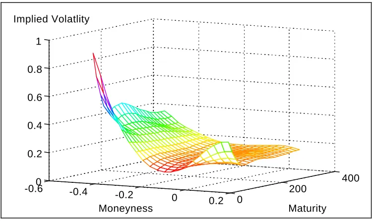
(37) Risk Management and Analysis: Measuring and Modelling Financial Risk. 37. (C. Alexander, Ed) Wileys, (1998). The Black-Scholes formula for the price of a call option with strike price K and time to maturity t on an underlying asset with current price S and t-period volatility σ is. (. C = SN ( x ) − Kr − t N x − σ t. ). (33). where r denotes the 'risk-free' rate of interest, N(.) is the normal distribution function and x = ln ( S / Kr − t ) σ t + σ t 2 . Option writers would estimate a statistical volatility and use the Black-Scholes or some other option model to price the option. But if C is observed from the market, and so also are S, K, r and t, then (33) may be used instead to ‘back-out’ a volatility implied by the model. This is called the (Black-Scholes) implied volatility, σ. Options of different strikes and maturities on the same underlying attract different prices, and therefore different implied volatilities. A plot of these volatilities against strike price and maturity is called the ‘volatility smile’ (see figure 13). Long term options have little variation in prices, but as maturity approaches it is typical that outof-the money options would imply higher volatility in the underlying than at-the-money options, otherwise they would not be in the market. Thus implied volatility is often higher for out-of-the money puts and calls than for at-the money options, an effect which is termed the ‘smile’. Equity markets exhibit a ‘leverage effect’, where volatility is often higher following bad news than good news (see section 4.3.2 (4)). Thus out-of-the money puts require higher volatility to end up inthe-money than do out-of-the money calls, and this gives rise to the typical ‘skew’ smiles of equity markets, such as in figure 13. The volatility smile is a result of pricing model bias, and would not be found if options were priced using appropriate stochastic volatility models (see Dupire, 1997). For example, when quantities are totally different: Implied methods assume risk neutrality and use a diffusion process for the underlying asset price..

(38) Risk Management and Analysis: Measuring and Modelling Financial Risk. 38. (C. Alexander, Ed) Wileys, (1998). options are priced using the Black-Scholes formula, which assumes log-normal prices, we observe volatility smiles because empirical returns distributions are not normal. Most noticeable in currency markets, returns distributions have much fatter tails than normal distributions, so out-ofthe money options have more chance of being in-the-money than is assumed under Black-Scholes. This underpricing of the Black-Scholes model compared to observed market behaviour yields higher Black-Scholes implied volatilities for out-of-the money options. Figure 13: Black-Scholes smile surface for FTSE options, December 1997 Figure 13: Smile surface of the FTSE, De 1. Implied Volatlity 1 0.8 0.6 0.4 0.2 0 -0.6. 400 -0.4. -0.2 Moneyness. 0. 200 0.2. 0. Maturity. ‘Volatility cones’ are graphic representations of the term structure of volatility, used for visual comparison of current implied volatility with an empirical historical distribution of implied volatilities. To construct a cone, fix a time to maturity t and estimate a frequency distribution of implied volatility from all t-maturity implied volatilities during the last two years (say), recording the upper and lower 95% confidence limits. Repeat for all t. Plotting these confidence limits yields a cone-like structure because the implied volatility distribution becomes more peaked as the option approaches maturity (see volume 1 chapter 8). Cones are used to track implied volatility over the life of a particular option, and under or overshooting the cone can signal an opportunity to trade. Sometimes cones are constructed on 'historic' volatility because historic data on implied.

(39) Risk Management and Analysis: Measuring and Modelling Financial Risk. 39. (C. Alexander, Ed) Wileys, (1998). volatility may be difficult to obtain. In this case cones should be used with caution, particularly if overshooting is apparent at the long end. Firstly, differences between long-term 'historic' and implied volatility are to be expected, since transactions costs are included in the implied volatilities but not the statistical. But also the ‘Black-Scholes bias, which tends to under price ATM options and over price OTM options, can increase with maturity. 4.4.2 Implied Correlation The increase in derivatives trading in OTC markets enables implied correlations to be calculated from three implied volatilities by rearrangement of the formula for the variance of a difference: if we denote by ρ the correlation between x and y σ x2− y = σ x2. or. ρ =. σ x2. + σ y2. − 2 σx σy ρ. + σ y2 − σ x2− y 2 σx σy. (34). Putting implied volatilities in formula (34) gives the associated implied correlation - we just need traded options on three associated assets or rates X, Y and X-Y. For example X and Y could be two US dollar FX rates (in logarithms) so X-Y is the cross rate. In the above formulae, the implied correlation between the two FX rates is calculated from the implied volatilies of the two USD rates σx and σy and the implied volatility of the cross rate σx-y . Similar calculations can be used for equity implied correlations: Assuming the correlation between all pairs of equities in an index is constant allows this correlation to be approximated from implied volatilities of stocks in the index - see Kelly (1994). Of course, the assumption is very restrictive and not all equities will be optionable, so the approximation is very crude and can lead to implied correlations which are greater than 1. Another way in which implied correlations can be obtained is by inverting the quanto pricing formula. When we know the quanto price, the interest rate, the equity and FX implied volatilities and so on we can invert the Black-Scholes quanto pricing formula to obtain an implied correlation between the equity and the FX rate..

No results found