Kernel Complexity for Nonparametric Distributions and Detection of Its Changes

(1)

Kernel Complexity for Nonparametric Distributions

and Detection of Its Changes

So Hirai1 _{* and Kenji Yamanishi}2

1

2

3

4

5

6

7

8

9

10

11

12

13

14

15

1 _Graduate_School_of_Information_Science_and_Technology,_The_University_of_Tokyo,_7-3-1_Hongo, Bunkyo-ku,Tokyo,Japan;[email protected]

2 _Graduate_School_of_Information_Science_and_Technology,_The_University_of_Tokyo,_7-3-1_Hongo, Bunkyo-ku,Tokyo,Japan;[email protected]

* Correspondence:[email protected]

Abstract: Thisstudyisconcernedwiththequantificationofstructuralinformationintheformof anindexfornonparametricdistributionswiththeaimofdetectingtheirchangesintimeseriesdata. In a parametric model suchas a Gaussian mixture model, thenumber of clusters canrepresent the structural information. However, the notion of structural information for modeling data nonparametricallydoesnotexist.Hereinweintroducethenovelnotionofkernelcomplexity(KC)as structuralinformationinanonparametricsetting.ThekeyideaofKCistocombinetheinformation bias by theGini indexwith the quantity ofinformation measured bythenormalized maximum likelihood(NML)codelength. WeempiricallyshowthesimilaritiesbetweenKCandthenumber of clusters in a parametric model under certain conditions. We propose an algorithm to detect structural changewith KCinnonparametric distributions. Usingsyntheticand realdatasets,we empiricallydemonstratethatourframeworkenablesustodetectthestructuralchangesunderlying thedata. Weusethesyntheticdatasetsto demonstratetheusefulness ofour methodwith some characteristic datadistribution. Wethen userealdatasetstoevaluatethevalidityofthedetected resultsbothquantitativelyandqualitatively.

Keywords: change-point detection; kerneldensity estimation; normalized maximum likelihood

(NML);minimumdescriptionlength(MDL)principle;kernelcomplexity(KC). 16

1. Introduction

17

1.1. Motivation 18

In this study, we define new structural information related to a nonparametric distribution and 19

propose a method to detect the changes in this distribution over time. The structure referred to 20

here is, for example, a cluster when a parametric model is employed for clustering purposes. The 21

number of clusters in a clustering model expresses structural information as a group of aggregated 22

data points. In contrast, as it is not possible to define a cluster in a nonparametric model, statistics 23

have previously been used to capture structures using the method of moments. However, even 24

in nonparametric distributions, it is important to aggregate structural information in the form of 25

data-like clusters to allow a global understanding of the data. In this study, we propose a new index 26

for structural information. This index, which we termed the kernel complexity (KC), defines the 27

structural information for a nonparametric model. The index is defined by using the Gini index to 28

measure the density of data in terms of information bias [1]. We measure the amount of information 29

provided by the data by determining the minimum description length (MDL), i.e., the shortest code 30

(2)

of the MDL principle [2], which asserts that the best way to model data is to select a model that 32

compresses the data and the model itself. Furthermore, we propose an algorithm to detect changes in 33

the KC when the data are in the form of a time series. This algorithm provides a framework for the 34

detection of changes based on the KC. 35

The data targeted in this research are provided as a time series, and we consider data that consist 36

of many multidimensional data points for each point in time. Situations that give rise to temporal 37

data such as these are e.g., customer purchases and sensor measurements. The ability to meaningfully 38

analyze these data would be useful for marketing purposes, for example. In the domain of marketing, 39

suppose we are given a sequence of datasets that contain a number of patterns of purchase behavior 40

that were observed over a period of time. Because user behavior changes as time passes, different 41

data distributions would be expected to appear as a result of the users’ actions. A dataset of which 42

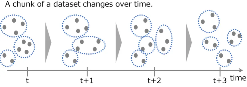
the structure changes as a function of time is illustrated in Figure1. 43

This study is concerned with detecting the changes the aforementioned data undergo without 44

assuming a specific distribution. Because we do not assume a specific parametric model, we consider 45

an approach that captures the changes in the distribution rather than observing the changes with 46

respect to the number of clusters. For this purpose, we use kernel density estimation as a way 47

to represent the data distribution. This approach enables us to even handle complex data chunks 48

that cannot be represented by parametric models. We calculate the index, KC, by making some 49

assumptions (e.g., by restricting the parameter on the normalized maximum likelihood (NML) 50

calculation, by restricting data structure, etc.). When capturing the changes in the distribution itself, 51

we apply the concept of clustering in a parametric model and propose a method to express the 52

complexity of the structure of the dataset in terms of the density of the dataset. In this case, the 53

amount of information used as a reference when capturing the overall image of the distribution would 54

be expected to differ between the high- and low-density sections of the dataset. Indexing the degree of 55

deviation of this information would then enable us to determine whether it is a complex distribution 56

(a state in which the dataset is sparsely distributed) or a plain distribution (a state in which the dataset 57

is densely distributed). It is possible to detect changes in the density distribution of data by observing 58

an index in a time series. For the purposes of this work, we formulate the following hypotheses for 59

considering changes in the data distributions. 60

• At a time when there is no change, the distribution maintains a certain form, and the index is 61

not observed to change. 62

• When the distribution changes, this change is considered to occur as a gradual transformation 63

from the original shape until it finally stabilizes as the changed shape. In the period during 64

which the change is undergoing transition, the index is also considered to gradually change 65

owing to the change in the distribution. 66

Under these hypotheses, we propose an index that quantifies the degree of information bias. In 67

addition, we propose a method that uses this index to detect the change from the perspective of the 68

distribution density. 69

This study has three aims. The first aim is to propose an index, named the KC, which defines 70

the structural information of a dataset. This index is defined as an indicator of the distribution of 71

peaks in the dataset similar to a cluster in clustering. The second aim is to develop an algorithm for 72

detecting changes in structure in a sequential setting. The third is to demonstrate the usefulness of 73

the proposed method by using two types of datasets, i.e., artificial and real practical datasets. 74

1.2. Related Work 75

We consider the related work from the viewpoints of both structural information and change 76

detection. To define structural information in terms of the density, the use of clustering methods 77

(i.e., aggregating data points into subgroups) is a well-known approach in parametric models (e.g., 78

(3)

Figure 1.Change in the structure of a dataset over time. The data points gradually move, causing the distribution of the dataset to gradually change.

moment method is a well-known method for defining the stochastic features to ultimately define the 80

structure of a nonparametric distribution [8]. Furthermore, the Kolmogorov complexity1[9] has long 81

been used as an index to indicate the complexity of data sequences. With reference to nonparametric 82

approaches for model selection, Zhang and K ˇosecká proposed a method to find the number of 83

regression lines [10]. A method that determines the number of clusters with kernel k-means was 84

proposed by Kyrgyzov et al. [11]. This method uses the information related to a latent variable 85

known as the cluster index. Our approach is to aim to quantify the global features of a distribution 86

without explicitly using the concept of clustering. 87

From the viewpoint of change detection, the changes undergone by models or parameters have 88

been detected by using various models that have been developed for this purpose. In the context 89

of parametric models, Herbster et al. proposed a method for tracking the best expert. This method 90

sequentially updates the weights of the models [12]. Erven et al. proposed the concept of a switching 91

distribution and a method for selecting a model in a situation in which the model changes over time 92

[13]. Yamanishi and Maruyama proposed a dynamic model selection (DMS) algorithm based on the 93

MDL principle to detect the changes in statistical models [14,15]. As an extension of this algorithm, 94

Hirai and Yamanishi proposed the sequential DMS (SDMS) algorithm, which is used to apply DMS to 95

a sequential setting [16]. Spiliopoulou et al. conducted research that adds a qualitative consideration 96

to the change in clustering by proposing a method to identify the nature of the transition of a cluster 97

on the basis of data movement between clusters [17]. 98

Methods that use nonparametric models have also been proposed. In the supervised scenario, 99

various methods based on the idea of concept drift have been developed [18]. Liu et al. proposed a 100

method based on estimation of the direct density ratio [19], and Jeske proposed a method referred to 101

as the CUSUM algorithm, which detects changes using the cumulative sum [20]. Tan et al. proposed 102

Bayesian change-point detection [21], which is a method based on the probability density. As a 103

nonparametric approach targeted by this research, Harchaoui et al. proposed an algorithm that 104

employs the kernel Fisher discriminant ratio [22], and Saatçi et al. proposed a method based on a 105

Gaussian process [23]. All of these methods detect changes based on the extent to which the data 106

distribution differs from that at a previous point in time. Our aim is to detect changes with respect to 107

the data aggregation by proposing changes in the values that quantify the structural information in 108

terms of the density. 109

(4)

1.3. Significance of This Study 110

The significance of this study is summarized as follows: 111

1. The proposal of an index to ascertain structural information without a specific probability

112

distribution

113

We propose an index named KC to ascertain the structural information of aggregated data. The 114

KC is defined by measuring the density of a dataset by determining the information bias with a 115

Gini index; a larger KC indicates that the distribution of the dataset is wider and the structure 116

is more complex. Rather than being a discrete value that indicates the number of clusters in a 117

parametric model, the KC is an index that takes continuous values. We can use KC as a new 118

quantitative indicator to ascertain nonparametric global information. 119

When using the KC, we especially use the NML code length based on the MDL principle as a 120

criterion to express information. The reason why we employ the NML code length is that it has 121

attractive properties: 122

(a) it minimizes Shtarkov’s minimax risk [24]. 123

(b) it optimizes the minimax estimation [25]. 124

Even though we adopt the kernel density estimation as a nonparametric density estimation 125

method, its NML code length cannot be directly calculated. This means we need to consider two 126

main points when calculating the NML code length. The first is to introduce a subprobability 127

distribution associated with the kernel density estimation. The second is to propose a method for 128

calculating the NML for this subprobability distribution by introducing a previously proposed 129

concept [26]. 130

2. The proposal of a method that uses KC to detect the points of structural change

131

In this paper, we propose an algorithm to detect the changes in KC when the data are given as 132

a time series. This makes it possible to detect changes in the global structure of nonparametric 133

data. 134

Many change-point detection algorithms for nonparametric distributions have been proposed 135

(e.g., [22,23]). In comparison, this algorithm only detects changes in the global information 136

measured by KC and provides a new view of nonparametric change detection. In addition, 137

KC does not always change suddenly; instead, it may experience gradual change. Because KC 138

is a continuous value, it is also able to detect such gradual change effectively. The use of KC 139

enables us to rank the time of interest by adding the degree of change to non-stationary time 140

series data. 141

3. Empirical validation of the usefulness of the proposed algorithm

142

In this study, we use simulation to empirically demonstrate the usefulness of the proposed 143

algorithm. In a simulation using artificial datasets, we find that the proposed algorithm can 144

calculate the degree of change and detect changes. In relation to the benefit, delay, false alarm 145

rate (FAR), and area under the curve (AUC) of the evaluation, the proposed algorithm was found 146

capable of detecting points of change earlier compared to other methods. 147

We empirically demonstrate that our algorithm can detect the changes in an actual dataset. That 148

is, our algorithm successfully processed: a dataset containing electricity consumption values to 149

detect high complexity at the time at which a change in lifestyle occurred; a dataset consisting 150

of sensor measurements to detect meaningful changes in the electric power consumption; a 151

dataset containing data pertaining to beer purchases to detect changes in customers’ purchasing 152

(5)

2. Criterion for Complexity of Dataset

154

2.1. Problem Setting 155

We consider a situation in which the distribution of the datasetXt, which is observed at each time 156

t, gradually changes over time. Each datasetXtcan be expressed asXt=xn = (x1,· · ·,xn)⊤∈Rn×m, 157

which consists ofndata points of dimensionm. For this purpose, we measure the density variation 158

as a complexity and detect change by detecting the change in density. 159

In this study, Xt is considered to have a complex distribution. Thus, we aim to define the structure of the dataset without using a specific parametric distribution. In this section, for brevity, we expressXt asX = xn = (x1,· · ·,xn)⊤ ∈ Rn×m. As we do not assume a specific parametric distribution, we use the following kernel density estimation:

f(x;h) = 1

n n

∑

j=1

K(x−xj;h),

whereK(·)is the kernel function, and we use the following Gaussian kernel:

K(x;h) = 1

(2πh2₎m/2exp {

− ||x||2 2h2

} .

2.2. Concept of the Proposed Method 160

Here we describe the concept of the proposed method. The degree of concentration of a dataset 161

at each time is expressed by focusing on the amount of information contained in each data point 162

included in the dataset. The amount of information represents the information associated with each 163

data point in defining a distribution. For example, we consider the density distribution in Figure2a. 164

The density distribution indicated by the solid blue line is expected to be defined by two high-density 165

peaks. Conversely, the structure of the density distribution indicated by the dotted orange lines can 166

be considered to be necessary to observe the structure of the density distribution by taking a wide 167

view of the data space. To understand the structure of the density distribution with the help of the 168

diagrams in the figure, an indicator would be useful to define a distribution as a complex distribution 169

when the information is widely distributed by measuring the amount of information contained in 170

the dense and sparse parts. For a sufficiently high density, we can think of an indicator that defines 171

a distribution as a dense (relatively easy) distribution. Then, we derive an index of the structural 172

information termed KC. 173

We measure the amount of information of the data in terms of MDL, i.e., the shortest code length 174

required to encode the data into a binary sequence in a prefix coding method. This is due to the 175

MDL principle [2], which asserts that the best way to model data is to use a model that compresses 176

both the data and the model itself. The MDL principle has been justified in a number of respects 177

such as consistency, rate of convergence (see e.g., [25]) in scenarios involving information theory and 178

statistics. In our setting, we employ Gaussian kernel density estimation as a nonparametric model of 179

the dataset. We then calculate the amount of information in terms of the NML code length of data 180

associated with the class of Gaussian kernel density. 181

The main process for defining KC can be expressed as follows: 182

1. We consider a subset of the dataset with constraints on the surrounding data where a certain or 183

higher data density is observed. We derive a parameterDdefined as the range of the subset. 184

2. We calculate the amount of information for the subset with NML code length. 185

3. We observe the change in the amount of information whenDis changed, and then express the 186

(6)

(a)Diagrammatic illustration of distribution complexity.(b)Plot of the amount of information (I(D)) versus the parameterD.

Figure 2.Visualization of the concept of KC.

2.3. Kernel Complexity 188

We propose an index that defines the complexity of a distribution in terms of its density. The index is illustrated in Figure2b. We hypothesize that KC is relatively small when data points are densely distributed (solid blue line). In contrast, KC is relatively large when data points are sparsely distributed (solid orange line). In Figure2b, the amount of information (denoted byI) increases with D. When the amount of information is biased for the data points in a specific dense area,Iis initially considered to increase significantly asDincreases, after which the change becomes gradual (see the blue line in Figure2b). In comparison, when the amount of information varies throughout the dataset, Iis considered to gradually increase asDincreases (see the orange line in Figure2b). In this way, this index can be understood as expressing the bias of the amount of information possessed by each data point. By using the Gini coefficient, which is used to express the extent to which data is biased in economics etc., this index can be formulated as follows:

KCdef= 1− ∫

DI(D)dD−12∆L·∆D−L0·∆D 1

2∆L·∆D

, (1)

whereI(D)is a function that defines the amount of information withD. 189

As the integral in equation (1) is difficult to calculate using actual data, we approximate it as follows:

∫

DI(D)dD≈_ℓp_≤

∑

_Dmax(ℓp−ℓp−1)I(ℓp),

(7)

2.4. NML Code Length associated with Kernel Density Estimation 191

In this section, we describe the NML code length, which we use as the definition of the amount 192

of information. Calculation of the NML code length associated with kernel density estimation is not 193

easy and it was therefore necessary to propose a method for this purpose. First, we describe the NML 194

code length as the code length of a dataset in Section2.4.1. In Section2.4.2, we derive a method for 195

calculating the normalization term of the NML code length proposed in [26]. In Section2.4.3, we 196

propose a new method for calculating the NML code length associated with the kernel density. 197

2.4.1. Normalized Maximum Likelihood 198

The NML code length is the optimal code length based on Shtarkov’s min–max criterion [24]. We first define the optimal model that satisfies the minimum NML code length. Let an observed data sequence be xn = (x1,· · ·,xn), wherexi = (xi1,· · ·,xim)⊤ (i = 1,· · ·,n). We use a model class P ={p(Xn;θ):θ∈Θ}. The NML code length for the data sequencexnis defined as follows:

L_NML(xn)def= −logp(xn; ˆθ(xn)) +logC(M),

whereC(M)is the normalization term and ˆθ(xn)is the maximum likelihood estimator calculated as follows:

C(M)def=

∫

p(yn; ˆθ(yn))dyn, ˆ

θ(xn)def= arg max θ p(x

n_;_θ₎_.

2.4.2. Calculation of the Normalization Term 199

Here we describe a method for calculating the normalization term of the NML code length, 200

which is generally difficult to calculate directly. Thus, we use the indirect method proposed by 201

Rissanen to perform this calculation [26]. In this method, when the maximum likelihood estimator of 202

the distribution parameterθis a sufficient statistic, it can be calculated analytically by the following 203

calculation method. 204

First, when the maximum likelihood estimator of the distribution parameterθ is a sufficient statistic, the distributionpcan be decomposed as follows:

p(yn;θ)dyn= f(z|θˆ)·g(θˆ;θ)dzd ˆθ

where we assume that a mapping q exists and we can write (θˆ,z) = q(yn), f is a conditional probability density function, andgis a probability density function of ˆθwhereθis a parameter. This equality allows us to calculate the normalization term as follows:

C(M)def=

∫

p(yn; ˆθ(yn))dyn =

∫ ∫

f(z|θˆ)·g(θˆ; ˆθ)dzd ˆθ

=

∫

g(θˆ; ˆθ)d ˆθ.

We use this method to calculate the NML code length associated with kernel density estimation. For 205

a detailed discussion, refer to the book published by Rissanen [26]. 206

2.4.3. NML Code Length associated with Kernel Density Estimation 207

(8)

length and kernel density estimation as a probability density distribution for a given dataset as follows:

f(x;h) = 1

n n

∑

j=1

K(x−xj;h),

where the functionK(·)is a kernel function. In the following discussion, we use the Gaussian kernel K(x;h) = 1/(2πh2)m/2exp{−||x||2/2h2}. Aiming to capture the structural changes, we consider calculating the likelihood using only the data points under the following conditions:

Ai =

{

j||xi−xj||2≤(1+γ)D }

(i=1,· · ·,n), (2)

B=

{ i _N1

(Ai)_j

∑

_∈_A_i||

xi−xj||2≤D }

, (3)

whereγ(>0)is a parameter. Under these conditions, we can derive the following theorem. 208

Theorem 1. The NML codelength for the subprobability disribution associated with kernel density is caluclated as follows:

nm 2 log

{

∑

i∈B

1

N(Ai)_j

∑

_∈_A_i||

xi−xj||2 }

−

_∑

i∈B (

m

m+4logn−mlogϵ )

+nmlog (

nm1+4

ϵ

)

+log log (

2πD·nm2+4 mϵ2

)

+nm

2 log(π)−logΓ (_nm

2 )

. (4)

Hereinafter, this NML code length is expressed as L_K₋_NML(xn;γ,D). 209

The proof has two parts. The first is the subprobability distribution we introduce with the 210

kernel density estimation. The second is a method we propose for calculating the NML for the 211

subprobability distribution associated with the kernel density estimation in Section 2.4.2. Details 212

of the calculation thereof are presented in AppendixA. 213

2.5. Kernel Complexity with the NML Code Length associated with the Kernel Density Estimate 214

We define KC by using the NML code length associated with the kernel density estimation, which is calculated in Section2.4.3. The definition of KC based on the NML code length is as follows:

KC_K₋_NML def= 1− ∫

DLK−NML(x

n_;_γ_,_D₎_dD₋1

2∆L·∆D−L0·∆D 1

2∆L·∆D

. (5)

Let us discuss the theoretical nature of the NML code lengthL_K₋_NML(xn;γ,D). This NML code length contains the hyperparametersγand D, and we evaluate the theoretical properties by tracking the change in the NML by Dfor fixed γ. First, we consider the case in which Dchanges by ∆DThe amount of change in the NML code length can be approximated as follows:

∆L=L_K₋_NML(xn;γ,D+∆D)−L_K₋_NML(xn;γ,D)

≈ nm 2 ·

1 1−δ·

N(∆B(D))

N(B(D)) , (6)

where N(B(D)) is the number of Bsets in equation (3), ∆B(D) is the increment of setB when D 215

changes by ∆D. Additionally, we define a parameter δ, 0 < δ < 1. Details of the calculation are 216

(9)

Equation (6) is proportional to the rate of increase inBsubject to the likelihood calculation. As 218

the value of∆Lindicates the extent to which the data points subject to the code length increase asD 219

increases, the width of the increase in the amount of information can be regarded as the amount of 220

information of the newly added data points. 221

2.6. Nature of KC 222

We calculated the value of KC for several generated datasets to evaluate the nature of KC. 223

Specifically, we evaluated the behavior of the values of KC with respect to the number of sets (clusters 224

in a parametric model) in the dataset and the behavior of the values of KC with respect to the extent 225

of the dataset. 226

2.6.1. Aggregated Dataset 227

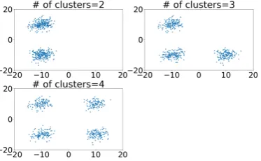
As a representative of a mixed dataset, we generated an artificial dataset, which we aggregated 228

into several chunks we refer to as clusters. We used the same artificial dataset and performed 229

the aggregation a few times to obtain a different number of clusters, and experimented with the 230

characteristics of the KC values for each of the datasets we produced in this way. The different 231

aggregations we generated are shown in Figure3. Using this dataset, we calculated the value of 232

KC, which is plotted in Figure4 as a function of the number of clusters. This result indicates that 233

KC increases as the number of clusters increases. Thus, from the viewpoint of data aggregation, 234

KC is considered to capture the characteristics of the structure of the distribution. In addition to these

Figure 3. Dataset aggregated into several chunks, which we refer to as clusters.

Figure 4. Value of KC as a function of the number of data chunks (clusters) in the dataset.

235

results, we also experimented with the behavior of KC by changing the dimensions of the dataset. The 236

results are shown in Figure5aand Figure5b. These results show that KC increases as the number 237

of clusters increases, and demonstrate the ability of KC to grasp the structural information of data 238

aggregation. 239

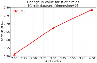
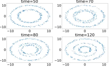
2.6.2. Circular Dataset 240

As nonparametric data cannot be expressed as a simple block, we investigated the characteristics 241

of KC of a dataset of which the data are aggregated into circular chunks (clusters). As before, we 242

varied the number of clusters, and investigated the extent to which the KC value depends on the 243

number of clusters. The dataset we generated is visualized in Figure 6. Using this dataset, the 244

calculated values of KC are plotted in Figure7as a function of the number of circles (i.e., clusters). 245

These results show that KC increases as the number of clusters increases; hence, KC is considered to 246

(10)

(a)Results for the dataset with a dimension of 3. (b)Results for the dataset with a dimension of 4. Figure 5.Value of KC for the dataset aggregated into several chunks (clusters) with a different number of dimensions.

Figure 6. Circular dataset with various numbers of clusters.

Figure 7.Value of KC for the circular dataset with aggregations into a different number of clusters.

3. Algorithm for Detecting Changes Using KC

248

Based on the above-mentioned findings, we proceeded to apply KC to further investigate its 249

ability to detect structural changes in a dataset. A dataset that undergoes structural change first 250

exhibits minor movement, after which a large change in the structure becomes visible. Because KC 251

is an index for evaluating the complexity of the distribution of a dataset, it can be considered as an 252

indicator of increasing complexity during substantial structural change. The algorithm we developed 253

to compute the KC index for structural change detection is presented in Algorithm1. For simplicity, 254

we express the dataset asXt∈Rn×mand expressKC_K₋_NML(Xt)asKCt. 255

4. Experimental Results

256

We empirically demonstrate the usefulness of the algorithm using both artificial and practical 257

(11)

Algorithm 1Algorithm for structural change detection.

Calculate KC:

Calculate KC score defined by equation (5) as follows:

KC_K₋_NML(Xt) =1− ∫

DLK−NML(Xt;γ,D)dD− 1

2∆L·∆D−L0·∆D 1

2∆L·∆D

.

Detection of changes:

Detect changes with following conditions:

a(t) =

{

1 if KCt−E[KCt−1]>η∗Std[KCt−1], 0 otherwise.

We can detect changes in the case wherea(t) =1.

4.1. Artificial Dataset for Change Detection 259

4.1.1. Circular Dataset 260

We generated an artificial dataset distributed on the circumferences of several circles and considered the case in which the number of circles gradually changes over time. The parameters of this dataset are defined as follows:

      

# of circles=K, r= (r1,r2) if 1≤t≤τ1, # of circles=K′, r= (r1,r2,u(t)) ifτ1+1≤t≤τ2, # of circles=K′, r= (r1,r2,r3) ifτ2+1≤t≤T,

(7)

whereu(t) = (τ2−t)r2+ (t−τ1)r3

τ2−τ1 ,

where the parameterrdenotes the radius of each circle. An example of the generated dataset is shown 261

in Figure8.

Figure 8. Dataset aggregated into circular data chunks over a period of time.

Figure 9. Calculated value of KC of the dataset aggregated into different circular chunks over time.

262

We found the points of change by using the index in Algorithm1. The results are shown in 263

Figure9, which shows that KC is able to detect a transition in the structure of the data over time and 264

(12)

In addition to the above qualitative interpretation, we calculated the benefit, delay, FAR, and AUC scores to evaluate the extent to which the algorithm could detect changes. The benefit, delay, FAR, and (area under the curve) AUC scores, respectively, are defined as follows:

benefitdef=

{

1−(tˆ−t∗)/U ift∗≤ˆt≤t∗+U,

0 otherwise; (8)

delaydef=

{ ˆ

t−t∗ if ˆt∈Transition period,

None otherwise; (9)

FARdef= #{tˆ∈/Transition period}

#{t∈/Transition period}, (10) AUCdef= Area under the curve created by plotting the benefit against the FPR. (11)

where ˆt is the first point at which the algorithm detects a change in the transition period or the 266

point at which the algorithm detects a change in any other period. In this study, the AUC is 267

calculated in relation to the benefit. Using these evaluation scores, we evaluated the proposed 268

algorithm in comparison with the density ratio estimation (DRE) algorithm [19], SDMS algorithm 269

[16], SE algorithm [27], tracking the best expert (TBE) algorithm [12], and the entropy-based method 270

(abbreviated as entropy), which is described in Algorithm2. When using the DRE algorithm, we 271

process the two-dimensional dataXt ∈ Rn×m at each time as one-dimensional dataX_t′ ∈ Rnm and 272

use them as the input for the DRE algorithm. Even though this is not a perfect fit for the model of 273

the DRE algorithm, it was added to the comparison as a model capable of detecting nonparametric 274

change. The point at which the data complexity begins to rise is defined as the starting point of change 275

in the model, and the proposed method was used to conduct a quantitative comparison experiment 276

using the value of KC. 277

Algorithm 2Entropy algorithm for detecting changes.

Calculate the density:

Calculate the density distribution as follows:

f(x; ¯h) = 1

n n

∑

i=1

K(x−xi; ¯h),

where we calculate the estimator ¯hon the basis of the method proposed by Scott [28], which is the default setting in the scipy.stats.gaussian_kde class (see [29]).

Calculate the entropy:

Calculate the entropy as follows:

Entropy=−

∫

f(y; ¯h(xn))logf(y; ¯h(xn))dy.

Detection of changes:

Detect the change points with following conditions:

a(t) =

{

1 if Entropyt−E[Entropyt−1_]_>_η_∗_Std_[_Entropyt−1_]_, 0 if otherwise.

The results are listed in Table1. We generated 10 different datasets with the same model and 278

detected the points of change for each dataset. The values provided in the table are the average values 279

of the benefit, delay, and FAR scores. These results show that the proposed algorithm (KC) can detect 280

the points of change to a certain extent in terms of the benefit and delay scores. Although the FAR 281

(13)

insignificant. Because the SDMS, SE, and TBE algorithms are based on a parametric Gaussian mixture 283

model (GMM), it is not possible to capture the changes in a circular distribution of data. The DRE 284

algorithm assumes that the data at each time consist of only a single scalar value; thus, it is difficult 285

to detect changes in this problem setting. 286

The main parameters of the generated data and algorithm are as follows. 287

• Dataset parameters: 288

We generated a circular dataset withK =2,K′ =3 clusters by using equation (7). The radii of 289

the circles werer= (10, 6, 3). A chunk of data starts its transformation at timet=50(=τ1+1) 290

and finishes forming a new chunk of data (a circle with radiusr=3) at timet=100(=τ2+1). 291

Each data point contains noise that follows a normal distribution with the standard deviation 292

σ=0.3. 293

• Algorithm parameters: 294

We used Algorithm1 to calculate the index to determine the points of change. The detection 295

parameter is η = 3, and the maximum value ofDis 100. In the evaluation, we defined the 296

parameterU =50 to calculate the evaluation scores and the length of the transition period as 297

50. 298

Table 1.Benefit, delay, and FAR scores for the algorithms (circle dataset).

Method Benefit Delay FAR KC 0.632 18.4 0.028 DRE 0.000 50.0 0.010 SDMS 0.000 50.0 0.000 SE 0.000 50.0 0.000 TBE 0.000 50.0 0.000 entropy 0.344 32.8 0.007

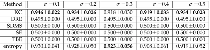
In addition to these results, we evaluated the experimental results by changing the noise level 299

(fromσ = 0.1 toσ = 0.5), focusing on the AUC scores. We calculated the AUC scores by changing 300

the detection parameterη(fromη=0.5 toη=3.0) in Algorithm1. We generated aggregations with 301

different patterns of the circular dataset with the following parameters: 302

1. The radii of the circles werer= (10, 6, 3). The new data chunk is a circle with the radiusr3=3. 303

The results are summarized in Table2. 304

These results are similar to those in Table1. On the basis of all the results, it is concluded that KC 309

is able to detect changes stably, regardless of the difference in the generation model and the value of 310

σ. The entropy method could detect changes with the next highest score. However, as described in 311

Section4.2, the entropy method requires computational time of an exponential order for the given 312

(14)

Table 2.AUC scores for the algorithms (circular dataset withr= (10, 6, 3)).

Method σ=0.1 σ=0.2 σ=0.3 σ=0.4 σ=0.5 KC 0.946±0.022 0.934±0.026 0.918±0.030 0.919±0.033 0.934±0.023 DRE 0.495±0.000 0.495±0.000 0.495±0.000 0.495±0.000 0.495±0.000 SDMS 0.500±0.000 0.500±0.000 0.500±0.000 0.500±0.000 0.500±0.000 SE 0.500±0.000 0.500±0.000 0.500±0.000 0.500±0.000 0.500±0.000 TBE 0.500±0.000 0.500±0.000 0.500±0.000 0.500±0.000 0.500±0.000 entropy 0.930±0.041 0.928±0.050 0.923±0.056 0.908±0.061 0.919±0.052

Method σ=0.1 σ=0.2 σ=0.3 σ=0.4 σ=0.5 KC 0.962±0.016 0.965±0.015 0.967±0.017 0.964±0.018 0.968±0.016 DRE 0.495±0.000 0.495±0.000 0.495±0.000 0.495±0.000 0.495±0.000 SDMS 0.500±0.000 0.500±0.000 0.500±0.000 0.500±0.000 0.500±0.000 SE 0.500±0.000 0.500±0.000 0.500±0.000 0.500±0.000 0.500±0.000 TBE 0.500±0.000 0.500±0.000 0.500±0.000 0.500±0.000 0.500±0.000 entropy 0.946±0.032 0.946±0.030 0.944±0.031 0.939±0.031 0.936±0.028

Method σ=0.1 σ=0.2 σ=0.3 σ=0.4 σ=0.5 KC 0.976±0.004 0.977±0.007 0.975±0.009 0.966±0.009 0.966±0.009 DRE 0.495±0.000 0.495±0.000 0.495±0.000 0.495±0.000 0.495±0.000 SDMS 0.500±0.000 0.500±0.000 0.500±0.000 0.500±0.000 0.500±0.000 SE 0.500±0.000 0.500±0.000 0.500±0.000 0.500±0.000 0.500±0.000 TBE 0.500±0.000 0.500±0.000 0.500±0.000 0.500±0.000 0.500±0.000 entropy 0.973±0.011 0.965±0.017 0.960±0.015 0.956±0.027 0.950±0.016

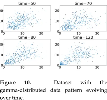
4.1.2. Gamma-Distributed Dataset 314

We generated an artificial dataset that follows the gamma mixture model and considered the case in which the number of mixtures gradually changed over time. The parameters of this dataset are defined as follows:

      

# of Gamma dist.=K, k= (k1,k2) if 1≤t≤τ1, # of Gamma dist.=K′, k= (k1,k2,u(t)) ifτ1+1≤t≤τ2, # of Gamma dist.=K′, k= (k1,k2,k3) ifτ2+1≤t≤T,

(12)

whereu(t) = (τ2−t)k2+ (t−τ1)k3

τ2−τ1

,

where the parameterkdenotes the shape of the gamma distribution. An example of the generated 315

dataset is shown in Figure10, which shows that data points that follow the gamma distribution with 316

k=1 are gradually generated over time. 317

We used Algorithm1to calculate the index to determine the points of change. The results are 318

shown in Figure11, which shows that KC gradually changes during the transition period and that it 319

(15)

Figure 10. Dataset with the gamma-distributed data pattern evolving over time.

Figure 11. Value of KC over time for the gamma-distributed data pattern.

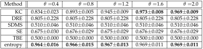
In addition, we evaluated the experimental results by changing the scale parameter (fromθ=0.4 321

toθ=2.0), by focusing on the AUC defined in equation11. We generated the dataset with the gamma 322

distribution with different data patterns, using the following parameters: 323

1. The shape parameters of the gamma distribution werek = (10, 5, 1). The new data chunk is a 324

cluster with the shape parameterk3=1. The results are summarized in Table5. 325

2. The shape parameters of the gamma distribution werek = (10, 1, 5). The new data chunk is a 326

3. The shape parameters of the gamma distribution arek = (1, 5, 10). The new data chunk is a 328

These results indicate that the value of KC and the entropy can be used to detect changes stably and 330

effectively. The DRE and SE produced relatively good results, confirming that the gamma-distributed 331

dataset is a model that easily enables both nonparametric and parametric changes to be detected. 332

It should be noted that the value of KC and the AUC scores for KC vary depending on the scale 333

parameter. This is probably because a constant value is used in this experiment. This suggests that 334

the integration range ofDshould be appropriately selected according to the data spread; this is left 335

for future study. In addition, the time required to calculate the entropy is of the exponential order 336

with respect to the data dimension; hence, in practice, the calculation is limited to two dimensions. 337

Therefore, this experiment was conducted using only two-dimensional data, and the behavior of KC 338

when processing high-dimensional data is left for future study. 339

Table 5.AUC scores for the algorithms (gamma dataset with shape parametersk= (10, 5, 1)).

(16)

Method θ=0.4 θ=0.8 θ=1.2 θ=1.6 θ=2.0 KC 0.965±0.018 0.900±0.005 0.939±0.031 0.977±0.006 0.878±0.036 DRE 0.858±0.133 0.858±0.133 0.858±0.133 0.858±0.133 0.858±0.133 SDMS 0.500±0.000 0.500±0.000 0.500±0.000 0.500±0.000 0.500±0.000 SE 0.848±0.003 0.849±0.005 0.849±0.004 0.848±0.003 0.848±0.003 TBE 0.500±0.000 0.500±0.000 0.500±0.000 0.500±0.000 0.500±0.000 entropy 0.917±0.021 0.915±0.023 0.905±0.025 0.905±0.027 0.904±0.027

Method θ=0.4 θ=0.8 θ=1.2 θ=1.6 θ=2.0 KC 0.834±0.023 0.893±0.005 0.945±0.009 0.973±0.008 0.969±0.009 DRE 0.805±0.228 0.805±0.228 0.805±0.228 0.805±0.228 0.805±0.228 SDMS 0.510±0.046 0.510±0.046 0.510±0.046 0.510±0.046 0.510±0.046 SE 0.675±0.030 0.676±0.029 0.675±0.029 0.676±0.029 0.676±0.029 TBE 0.500±0.000 0.500±0.000 0.500±0.000 0.500±0.000 0.500±0.000 entropy 0.964±0.016 0.966±0.015 0.967±0.013 0.969±0.011 0.969±0.011

4.1.3. Cross Dataset 340

We generated an artificial dataset distributed along straight lines for several chunks of data points and considered the case in which the number of chunks gradually changed over time. The parameters of this dataset are defined as follows:

# of lines=K(1≤t≤T), a= (a1,u(t)) (1≤t≤T), u(t) = (T−t+1)·a1+ (t−1)·a2

T .

We generated an artificial dataset withK = 2, a1 = −0.95, anda2 = 0.95, where the parameter a 341

denotes the slope of a straight line. An example of the generated dataset is shown in Figure12, which 342

shows that one of the straight lines is gradually rotating over time. 343

We used the index in Algorithm 1 to detect the points of change. The results are shown in 344

Figure 13, which indicates that KC is gradually decreasing. This is because the density of the 345

distribution at the center of the distribution becomes relatively larger owing to the gradual movement 346

of one of the straight lines, with an accompanying decrease in the complexity. 347

In addition, we evaluated the experimental results by changing the noise level (fromσ=0.5 to 348

σ=2.5), by focusing on AUC defined in equation11.

Table 8.AUC scores for the algorithms (cross dataset).

Method σ=0.5 σ=1.0 σ=1.5 σ=2.0 σ=2.5 KC 0.908±0.007 0.912±0.005 0.846±0.026 0.915±0.012 0.914±0.013 DRE 0.495±0.000 0.495±0.000 0.495±0.000 0.495±0.000 0.495±0.000 SDMS 0.613±0.018 0.495±0.005 0.500±0.000 0.500±0.000 0.500±0.000 SE 0.615±0.029 0.500±0.022 0.500±0.000 0.500±0.000 0.500±0.000 TBE 0.582±0.019 0.500±0.000 0.500±0.000 0.500±0.000 0.500±0.000 entropy 0.782±0.000 0.500±0.000 0.877±0.006 0.871±0.001 0.808±0.015

(17)

Figure 12. Dataset with data chunks in the form of a cross.

Figure 13. Value of KC over time for the dataset with datachunks in the form of a cross pattern.

Considering the overall results, KC is able to detect changes stably, regardless of the difference 350

in the value ofσ. For small values ofσ, the methods based on parametric models (the SDMS, SE, and 351

TBE algorithms) were sometimes able to detect the points of change, probably because the dataset is 352

relatively closely approximates a GMM. 353

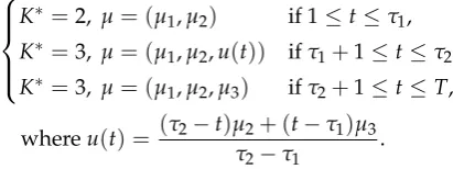
4.1.4. Gaussian Mixture Model 354

We generated an artificial dataset distributed using a GMM, of which the parameters are defined as follows:

      

K∗=2, µ= (µ₁,µ2) if 1≤t≤τ1, K∗=3, µ= (µ1,µ2,u(t)) ifτ1+1≤t≤τ2, K∗=3, µ= (µ1,µ2,µ3) ifτ2+1≤t≤T,

(13)

whereu(t) = (τ2−t)µ2+ (t−τ1)µ3

τ2−τ1

.

A chunk of data starts undergoing transformation at timet= 50 and finishes forming a new chunk 355

of data at timet=100. An example of the generated dataset is shown in Figure14.

Figure 14. Dataset aggregated into data chunks using the Gaussian mixture model.

Figure 15. Value of KC over time for the dataset aggregated using the Gaussian mixture model.

356

We used the index in Algorithm1to detect the change points. The detection parameter isη=3 in 357

Figure15. During the transition period, KC gradually increases at first, then gradually decreases after 358

reaching its peak, before stabilizing in a certain range. Points of change are indicated by a gradual 359

(18)

We also generated datasets by changing the variance of the Gaussian model fromσ2 = 2.0 to 361

σ2 ₌_{10.0. The resultant AUC scores (see equation}_{11) are listed in Table}_{9. KC was able to indicate} 362

points of change earlier than the other methods assuming a GMM (SDMS, SE, and TBE algorithm) 363

because it captures changes in the density distribution. In models that assume a GMM (SDMS, SE, 364

and TBE algorithm), the number of clusters changes to a certain degree at a time when a chunk of 365

the dataset undergoes transformation. In contrast, KC can be considered to indicate change in the 366

complexity from the point at which a chunk of the dataset starts to gradually transform. Because of 367

these characteristics, the nonparametric KC could detect change at the earliest time. 368

Next, we observed the behavior of the benefit and FAR scores when calculating the AUC for 369

different values of the sensitivity parameter. The results are shown in Figure16, which indicates 370

that KC yields high benefit values, but the corresponding FAR values are also relatively high. This is 371

attributed to KC being more sensitive to change than the other methods. The results in the figure show 372

that each algorithm becomes less sensitive to change as the change sensitivity parameter becomes 373

larger (the change is judged more severely). For SDMS and TBE, which contain no sensitivity 374

parameters, the scores of benefit and FAR were constant. The SE algorithm would be expected 375

to enable change to be detected outside the transition period by reducing the change sensitivity 376

parameter. The values of benefit could be considered to be low because the subsequent time is not 377

detected as a change. 378

Observing the curve plotting benefit against FAR as shown in Figure17, the AUC score of KC 379

was higher because the advantages of benefit exceed the disadvantages of FAR. 380

Table 9.AUC scores for the algorithms (GMM dataset).

Method σ2₌_2.0 _σ2₌_4.0 _σ2₌_6.0 _σ2₌_8.0 _σ2₌_10.0 KC 0.943±0.028 0.965±0.014 0.951±0.018 0.924±0.047 0.930±0.037 DRE 0.495±0.002 0.495±0.002 0.493±0.006 0.493±0.008 0.492±0.009 SDMS 0.667±0.187 0.656±0.136 0.731±0.184 0.520±0.065 0.567±0.121 SE 0.813±0.095 0.784±0.165 0.787±0.157 0.810±0.132 0.714±0.170 TBE 0.636±0.167 0.589±0.147 0.619±0.135 0.500±0.000 0.489±0.010 entropy 0.584±0.178 0.922±0.031 0.921±0.034 0.913±0.030 0.914±0.037

Figure 16. Evaluation of KC vs. the other algorithms by plotting benefit and FAR against the change sensitivity parameter.

Figure 17. Evaluation of KC vs. the other algorithms by plotting the benefit against FAR.

4.2. Calculation Time 381

We evaluated the calculation time of KC and the entropy used above with a number of different 382

dimensions. We used the dataset with the same settings as in Section 2.6.1. To complete the 383

(19)

are shown in Figure 18, which shows that the time required to compute KC is independent of 385

the dimension. However, the time required to calculate the entropy increases exponentially as the 386

dimension increases.

Figure 18.Time required by the two methods to perform the calculation for different dimensions. 387

4.3. Real Datasets 388

4.3.1. Sensor Dataset (Household Electricity Consumption) 389

Figure 19.KC at each time (household).

Figure 20. Average consumption of the first feature (in the kitchen and laundry room) for each week.

We tested our method by using a dataset comprising household electricity consumption 390

measurements provided by Dua and Graff [30]. This dataset contains three categories of electricity 391

consumption data: 1. by the kitchen and laundry room, 2. by an electric water heater, 3. by the air 392

conditioner. The data were acquired every other minute from December 17, 2006 to December 10, 393

(20)

the value of the total consumption in an hour for each of the three categories, and eachXtrepresents 395

the consumption for one week (the number of datasets at each time wasn=168 or less). 396

The results obtained with the proposed method enabled us to observe changes in the data 397

sequence at a specific time. The value of KC is shown in Figure19as a function of time. We could 398

detect large changes att=87, 88 (August 17–23, 2008 and August 24–30, 2008). As seen in Figure20, 399

the use of electricity in the kitchen and laundry room on a normal day is always greater than zero; 400

however, the consumption is zero for the week in which the change is detected. This is because we 401

were able to observe some lifestyle anomalies (or changes) by calculating the value of KC. 402

4.3.2. Marketing Dataset (Beer Purchasing Behavior) 403

Figure 21.KC at each time (beer).

We tested our method using a dataset containing data of beer purchases that was provided 404

by Hakuhodo, Inc. and M-CUBE, Inc. QPR. The dataset is a record of customers’ beer purchasing 405

behavior and includes brands from six manufacturers (denoted A–F here). We captured the changes 406

in the requirements of high-value customers by using simulation and analyzed the data using the top 407

50% of customers in terms of purchasing volume. The dataset at each instant represents the amount 408

purchased for the four categories of beer in the last two weeks, where the target period was from 409

November 1 to January 31 of the following year. 410

The results obtained with the proposed algorithm to calculate the value of KC to detect the 411

points of change are shown in Figure21. The proposed algorithm detected points of significantly 412

large change on December 1, 3, and 31 and on January 1, 13, 14, and 15 (time=17, 19, 47, 48, 60, 61, 62). 413

The detection of change in customers purchasing behavior in the last two weeks of November and 414

December reflects the year-end demand, and the complexity of the structure decreases because the 415

beer consumption stabilizes after the end of the year. These results confirm the ability of the proposed 416

(21)

5. Conclusion

418

This paper proposed a method to calculate the value of KC to define new structural information 419

for data with a nonparametric distribution and proposed a method to detect its change over time. 420

This index is defined by measuring the density of data in terms of information bias and is based on 421

the Gini index. We use the NML code length based on the MDL principle as a criterion to express 422

information. We showed that this index, KC, is a value that characterizes the number of data chunks. 423

Furthermore, we proposed an algorithm to detect the change in KC when the data are given as time 424

series. By using this algorithm, we provide a framework for the detection of changes based on KC. 425

However, KC has some limitations. First, since the parameters that define KC are not determined 426

with theory, it is a future research issue to improve the reliability of KC by establishing parameter 427

determination theory. Second, the assumed data structure is a structure with data chunks, and the 428

usefulness of KC has only been shown in experiments focusing on the number of data chunks. For 429

this reason, we consider that application to other data structures or proposal of new methods is a 430

future research issue. 431

The usefulness of the proposed method was experimentally demonstrated using both artificial 432

and real datasets. For the artificial datasets, the proposed algorithm could detect the change points 433

in terms of the benefit, delay, FAR, and AUC scores for specific kinds of datasets. Further, we 434

showed the effectiveness of our method for analyzing a dataset containing household electricity 435

consumption data. Specifically, our algorithm automatically detected changes at times when the 436

electricity consumption in the kitchen and laundry room was likely to change. In addition, we also 437

analyzed a dataset containing data relating to customers’ beer purchasing behavior over time. The 438

purchasing behavior significantly changed over the last part of the year and after the year ended, and 439

the proposed algorithm effectively captured these changes. 440

The ability of the proposed method to capture the complexity in a data structure that can be 441

defined by the density has expanded the possibility of searching for new hidden value. In future, we 442

aim to extend our work to other kernel functions, and to calculate exact values rather than the upper 443

bound in the form of the NML. With respect to the KC index itself, analysis of the theoretical nature 444

of this indicator (e.g., its properties by using the Gini coefficient) remains as an extension of current 445

research. This may enable us to obtain appropriate values for the parameters (the features of the KC 446

index depend on the parameters to some extent). In terms of applications, we consider adding more 447

qualitative interpretations of actual data in combination with other methods. In addition, considering 448

the application of our method, real data are rarely neatly arranged; thus, extending KC to an index 449

that can handle missing data is a very important issue. 450

Author Contributions: conceptualization, S.H. and K.Y.; methodology, S.H.; software, S.H.; validation, S.H. 451

and K.Y.; formal analysis, S.H.; investigation, S.H. and K.Y.; resources, S.H.; data curation, S.H.; writing–original 452

draft preparation, S.H. and K.Y.; writing–review and editing, S.H. and K.Y.; visualization, S.H.; supervision, K.Y.; 453

project administration, K.Y.; funding acquisition, K.Y. 454

Funding:This work was partially supported by JST KAKENHI 191400000190 and JST-AIP JPMJCR19U4. 455

Acknowledgments:The marketing dataset was provided by Hakuhodo Inc. and M-CUBE, Inc. QPR. 456

Conflicts of Interest:The authors declare no conflict of interest. 457

Appendix A Calculation of the NML Code Length with Subprobability Distribution associated

458

with Kernel Density Estimation

459

First, we consider a bandwidth estimator with the kernel density function. We derive the log-likelihood as follows:

logf(xn;h) =−

∑

i∈B log

(

N(Ai)(2πh2)

m

2 )

+

∑

i∈B log

∑

j∈Ai

exp {

− 1

2h2||xi−xj|| 2

(22)

where N(Ai)and N(B) are the number of Ai and B sets, respectively. Then, using the inequality log

( 1 n∑ni=1xi

) ≥ 1

n∑ni=1logxi, the lower bound of this log-likelihood can be calculated as follows:

logf(xn;h) =−

∑

i∈B log

(

(2πh2)m2 )

+

∑

i∈B log

( 1 N(Ai)_j

∑

_∈_A_i

exp {

− 1

2h2||xi−xj|| 2

})

≥ −

_∑

i∈B

log((2πh2)m2 )

−

_∑

i∈B 1 N(Ai)_j

∑

_∈_A

i

1

2h2||xi−xj||

2_. _(A1)

The bandwidth h of a kernel density was optimized to be h = O(n−1/(m+4)) in the past work (e.g., refer to [28]) so that the generalization error for the maximum likelihood estimator for h is minimal. When considering the NML code length associated with the kernel, we set a constraint ofh ≥ ϵ·n−1/(m+4)/√2π using a positive constantϵ. Under this condition, equation (A1) can be lower-bounded as follows:

Equation(A1)

= −N(B)log (

(2πh2)m2 )

−

_∑

i∈B 1 N(Ai)_j

∑

_∈_A_i

1

2h2||xi−xj|| 2

= −N(B)log ((

2πh2·nm2+4 · 1

ϵ2 )m

2 )

−

_∑

i∈B {

1 N(Ai)_j_∈

∑

_A_i

1

2h2||xi−xj||

2₋ m

m+4logn+mlogϵ }

≥ −nlog ((

2πh2·nm2+4 · 1

ϵ2 )m

2 )

−

_∑

i∈B {

1 N(Ai)_j

∑

_∈_A_i

1

2h2||xi−xj||

2₋ m

m+4logn+mlogϵ }

=: ˜L(xn;h). (A2)

Then, we calculate the estimator ˜hsuch that ˜L(xn;h)is maximized as follows:

˜ h(xn) =

√ 1 nm_i

∑

_∈_B

1 N(Ai)_j

∑

_∈_A

i

||xi−xj||2.

We define the distribution ˜f as follows: ˜

f(xn;h)

def

= exp{L˜(xn;h)}

= ₍ 1

2πh2·_nm2+4 · 1 ϵ2 )nm 2 exp { − 1

2h2

∑

i∈B

1 N(Ai)_j

∑

_∈_A

i

||xi−xj||2 }

×exp {

∑

i∈B

( m

m+4logn−mlogϵ )}

.

Using this equation and equation (A2), we find that the distribution ˜f is a subprobability distribution by the following formula:

∫ ˜

f(xn;h)dxn≤

∫

f(xn;h)dxn=1.

Then, the NML distribution of ˜f can be calculated as follows:

˜

f_NML(xn)def= f˜(x

n_{; ˜}_h₍_xn₎₎

C ,

Cdef

=

∫ ˜

(23)

whereC is a normalization term of the NML distribution. In general, the normalization term cannot be calculated in a straightforward manner; instead, we calculate this term using the method described in Sec.2.4.2. We can decompose ˜f(xn;h)as follows:

˜

f(xn;h)dxn= f¯(z|h˜)·g(h;˜ h)dz ˜h,

where the function g is the gamma distribution with the shape parameter k = nm/2 and scale parameterθ=2h2/nm:

g(h;˜ h) = 2˜h

Γ(nm

2 ) (_2h2

nm )nm

2 (

˜ h2

)nm

2 −1 exp

{ − h˜2

2h2_/nm }

.

Then, we can define

g(h˜)def= g(h; ˜˜ h) = 2 exp

( −nm

2 )

Γ(nm

2 ) ( ₂

nm )nm

2 · 1

˜ h.

Then, we can calculate the normalization termCfor integrating with respect to ˜has follows: C=

∫

Y ˜

f(yn; ˜h(yn))dyn

=

∫ √_D/m

ϵ·n−1/(m+4)_/√₂_πg(

˜ h)d˜h

= 2 exp

( −nm

2 )

Γ(nm

2 ) ( ₂

nm )nm

2 ·log  

√

2πD·nm2+4 mϵ2

 _,

where we define the range of ˜h asY = [1/√2π,√D/m]. The upper bound on ˜h is calculated as follows:

˜ h(xn) =

√ 1 nm_i

∑

_∈_B

1 N(Ai)_j

∑

_∈_A

i

||xi−xj||2

≤ √

1 nm_i

∑

_∈_BD ≤