Source parameters of the 2007 Noto Hanto earthquake sequence derived from
strong motion records at temporary and permanent stations
Takahiro Maeda1, Masayoshi Ichiyanagi1, Hiroaki Takahashi1, Ryo Honda1, Teruhiro Yamaguchi1, Minoru Kasahara1, and Tsutomu Sasatani2
1Institute of Seismology and Volcanology, Graduate School of Science, Hokkaido University, N10W8 Kita-ku, Sapporo 060-0810, Japan 2Graduate School of Engineering, Hokkaido University, N13W8 Kita-ku, Sapporo 060-8628, Japan
(Received June 30, 2007; Revised December 6, 2007; Accepted January 8, 2008; Online published November 7, 2008)
A large crustal earthquake, the 2007 Noto Hanto earthquake, occurred west off the Noto peninsula in Ishikawa prefecture, Japan, on March 25, 2007. We started temporary strong motion observation at five sites within the aftershock area from about 13 h after the main shock occurrence. We first applied the spectral inversion method toS-wave strong ground motion records at the temporary and permanent stations. We obtained source specta of the main shock and aftershocks,Qs(quality factor forS-wave) values (Qs=34.5f0.95) and site responses at 22 sites. We then estimated a source model of the main shock using the empirical Green’s function method. The source model consists of three strong motion generation areas and well explains the observed records. Finally, we examined the consistency of the main-shock source models estimated from the above two analyses. The high-frequency level of the acceleration source spectrum based on the main-shock source model is consistent with the source spectrum estimated from the spectral inversion. The combined area of strong motion generation areas is approximately half of the value expected by the empirical relationship, and the high-frequency level of acceleration source spectrum is approximately 2.5 times larger than the empirical relationship for shallow inland and inter-plate earthquakes.
Key words: 2007 Noto Hanto earthquake, temporary strong motion observation, spectral inversion method,
empirical Green’s function method.
1.
Introduction
A damaging large crustal earthquake, the 2007 Noto Hanto earthquake, occurred west off the Noto peninsula in Ishikawa prefecture at 0941 hours on March 25, 2007 (JST). The moment magnitude (MW) determined by the
F-net Project of National Research Institute for Earth Science and Disaster Prevention (NIED) is 6.7. The focal depth and magnitude (MJ) determined by Japan Meteorological
Agency (JMA) are 10.7 km and 6.9, respectively. A max-imum seismic intensity of 6 upper in the JMA scale was observed at some stations around the epicenter. This earth-quake caused widespread destruction: one person died, 359 persons were injured, and 15,757 houses were damaged as of June 14 (Fire and Disaster Management Agency, 2007).
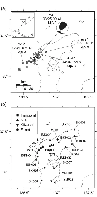
We made an urgent strong motion observation at five sites within the aftershock area from 25 March to 14 May, 2007 (Fig. 1, Table 1). An accelerometer type strong motion seis-mograph (JEP-6A3, Mitsutoyo Co.) was installed at each observation site and seismic data were recorded continu-ously in a data logger (LS7000XT, Hakusan industry) at 100 sample/second.
In this paper, we estimate source parameters of the main shock and aftershocks, Qs values and site responses by applying the spectral inversion method to strong-motion
Copyright cThe Society of Geomagnetism and Earth, Planetary and Space Sci-ences (SGEPSS); The Seismological Society of Japan; The Volcanological Society of Japan; The Geodetic Society of Japan; The Japanese Society for Planetary Sci-ences; TERRAPUB.
data at the temporary and permanent stations. We then estimate a main-shock source model using the empirical Green’s function method. Finally, we examine the scaling of source parameters and the consistency of the main-shock source spectra deduced from the above two analyses.
2.
Estimation of the Source, Path, and Site Effects
Observed S-wave spectrum O(f) is expressed asO(f) = S(f)G(f)R−1exp(−πf T/Qs(f)), where R is the hypocentral distance, R−1 represents a geometrical
spreading, andTis anS-wave travel time. We assume a ge-ometrical spreading effect for the body wave, because theS -wave is dominant in analyzing time windows. Source spec-tra S(f), path-averaged quality factor for S-wave Qs(f), and site responsesG(f)are estimated using strong ground motion records at the temporary and permanent stations. A spectral inversion method (Iwata and Irikura, 1988; Maeda and Sasatani, 2006) is adopted to the observedS-wave spec-tra from the main shock and small events. Two linear in-equality constraints (G(f)≥2 andQ−s1(f)≥1000−1f−1) are applied to the inversion. The former (G(f) ≥ 2) rep-resents the free surface amplification effect and removes a trade-off problem between S(f) and G(f) (Iwata and Irikura, 1988).
S-wave Fourier amplitude spectra are calculated using Fast Fourier Transform. The time window for the analysis is 10.24 s for the main shock and 5.12 s for the small events; a cosine-shaped taper at 10% each end of the window is
Table 1. The temporary observation stations.
Station Latitude Longitude Observation period Site condition∗
MNZ 37.2922 136.7603 3/25, 22:45–5/14 Alluvial deposits
CHY 37.2681 136.7361 3/25, 23:00–5/14 Miocene conglomerate
URK 37.3083 136.7935 3/26, 10:10–5/14 Alluvial deposits
KOT 37.2307 136.7102 3/26, 16:00–5/14 Miocene andesite lava MTI 37.3166 136.8996 3/27, 11:15–5/14 Miocene andesite lava
∗Geological Survey Japan (1967).
(a)
(b)
ev01 03/25 09:41
Mj6.9
ev21 03/25 18:11
Mj5.3 ev25
03/26 07:16 Mj5.3
ev45 04/06 15:18
Mj4.3
Fig. 1. Location map of epicenters and stations used in this study. (a) Star is epicenter of the 2007 Noto Hanto earthquake. Open circles are earthquakes used in the spectral inversion; solid circles are the aftershocks. Epicenters are taken from the JMA unified catalogue. The focal mechanism solution of the main shock determined by the F-net is shown. The study area is shown by a square in the inset map. (b) Solid symbols represent temporary and permanent strong-motion stations.
plied. To equalize a frequency interval, an extra 5.12 s with zero value is added to the small-event records. A moving average of±1/5f0 window (f0, central frequency) is
ap-plied as a smoothing of amplitude spectra; the 25 central frequencies are chosen as they are distributed at a common interval from 0.1 to 20 Hz logarithmically. The vector sum-mation of two horizontal component spectra is used for the inversion. Data with a signal-to-noise ratio greater than 2 at each frequency are used for the inversion; noise spectra are calculated using a seismogram just before the S-wave arrival. The frequency band to analyze is limited (about
ISK002 ISKH01
CHY URK WJM ISK006 ISKH06 ISK003 ISKH02 ISK004 TYM002 ISK001
KOT MNZ MTI ISKH04 ISK005 ISKH05 ISK007 ISK008 TYMH01 ISKH03
0
Travel time (s) 20 10
Fig. 2. TheS-wave travel time distribution of data used in the spectral inversion. Circles are data from the main shock and aftershocks, and crosses are those from the additional events.
0.5–20 Hz) due to the low signal-to-noise ratio of the data. We analyzeS-wave spectra from the main shock and 37 aftershocks (MJ: 3.3–5.3, depth: 0–13.5 km) at 22 stations
in the Noto peninsula (Fig. 1) (dataset 1). The location, ori-gin time, and magnitude of these events are taken from the JMA unified catalogue. The 22 stations consist of nine K-NET, seven KiK-net, one F-net, and five temporary stations. We use data with peak horizontal amplitudes of less than 100 cm/s/s in order to avoid an influence of nonlinear site response. Although observed records of the main shock at the stations shown in Fig. 1 exceed 100 cm/s/s, we use data at far-fault stations (ISK001, ISK002, ISK008, TYM002, ISKH01, ISKH02, WJM) for the inversion. Data having an
S-wave travel time larger than 5 s are also used (Fig. 2). Figure 3 shows the estimatedQs values, source spectra, and site responses (bold dotted lines). The site response at WJM equals 2 for most of frequencies and, therefore, WJM is a reference site of the inversion; this is a reason-able result, since WJM is placed in a vault. Theoretical site responses for the K-NET and KiK-net stations, where log-ging data are available, are shown in Fig. 3(c). Site response is evaluated using the Propagation Matrix method (Aki and Richards, 1980) for a vertical incident SH wave. A pre-dominant frequency of the estimated site response with a steep spectral peak agrees with that of the theoretical site response (i.e. ISK005). In contrast, the amplitude of the es-timated response is larger than that of the theoretical one; this is probably the effects of a deep structure from a base-ment, corresponding to a WJM site, to a logging-data depth; the logging-data depths are up to about 20 m and 200 m for the K-NET and KiK-net, respectively.
cm/s
(a)
(c)
(b)
Qs
value
ev01: 07/03/25 09:41 ev21: 07/03/25 18:11 ev25: 07/03/26 07:16 ev45: 07/04/06 15:18
f 4.14 (Hz) f 8.64 (Hz) m 2.9
c max M 1.06E+150 (Nm)
M 7.52E+16(Nm) f 0.72 (Hz) f 7.92 (Hz) m 2.8
0 c max M 5.32E+16
f 0.90 (Hz) f 10.00 (Hz) m 3.3
0 c max
(Nm)
f 7.57 (Hz) m 3.2
max
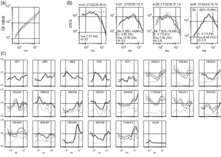
Fig. 3. Results of the spectral inversion. (a)Qs values, (b) acceleration source spectra for selected events, and (c) inverted site responses. Bold, thin and dotted lines are the results from inversion of the data subsets (dataset 3), all available data (dataset 2), and data on the main shock and aftershocks (dataset 1), respectively. Theoretical source spectra and site responses are shown by a thin dotted line. The high-frequency level of the main-shock acceleration source spectrum (ev01) based on fault parameters of the strong motion generation areas (Fig. 5) is shown as a broken line.
stations farther from the aftershock area have a larger am-plification. This distance dependency may arise from a spe-cific configuration of stations and earthquakes; the after-shock area is small compared with the extent of stations (Fig. 1). In this case, observed data at each station have ap-proximately the same hypocentral distance and travel time (Fig. 2) and, therefore, a reliability in the estimate of the
Qs value and site response may decrease. To maintain a wide travel-time range for each station, nine events occur-ring around the Noto peninsula are added to the data set (open circles in Fig. 1(a);MJ: 3.7–4.8, depth: 6.7–19.3 km).
This new data set (dataset 2) provides a wide travel-time range for the permanent stations (Fig. 2). We also make data subsets to decrease the contribution of the aftershocks to the inversion results as follows.
The 47 events (total) are divided into two groups; Group A includes the main shock and nine events occur-ring outside of the aftershock area, and Group B includes 37 aftershocks. The inversion analysis is performed using 100 data subsets (dataset 3). Each data subset includes 20 events: ten events from Group A and another ten events ran-domly selected from Group B. The final result (Fig. 3; bold lines) is an average of the 100 inversion results; source spec-tra from Group B are averages of 19–38 models, depending on a random selection. Standard deviations of the results are very small and, therefore, not shown in the figure.
Qsvalues estimated from dataset 3 are larger than those from the dataset 1. The site responses at the near aftershock
area (i.e. ISK006) increase using dataset 3, while those far from the aftershock area (i.e. ISK001) decrease. On the other hand, the source spectra are stable and independent of the data sets. These facts indicate that the trade-off problem betweenQs(f)andG(f)is reduced using the data subsets. We fit a power law to the frequency dependence of Qs values for the frequency band 1–10 Hz and obtain Qs = 34.5f0.95. In the same region, Kato and Ikeura (2007) obtained Qs =30f1.2using the spectral inversion method. These reserchers used strong ground motion data from the main shock and aftershocks and gave a constraint condition on source spectra. OurQs values estimated from the main shock and aftershocks (dataset 1) are expressed as Qs = 25.6f0.86. A part of the discrepancy may result from the
different constraint conditions.
Figure 3(b) shows a part of the estimated source spectra together with the theoretical ones. The theoretical displace-ment spectraM(f)based on theω−2model are represented
as
M(f)=M0
1 1+(f/fc)2
1 1+(f/fmax)m
, (1)
where M0 is a seismic moment, fc is a corner frequency, and fmax is a high-frequency cutoff of the source
spec-trum. We adapt the method of Andrews (1986) for a fi-nite frequency band (0.5–5 Hz) to determine fc and flat level of source displacement spectrum0from the inverted
source spectra. Seismic moment is calculated from 0; M0 =4πρsβs3R00/Rθφ
100
MPa 0.1
MPa 1
MPa 10
MPa (a)
(c) (b)
Fig. 4. (a) Relation between the seismic moment (M0) determined in this study and that determined by F-net, (b)M0-fc(corner frequency) relation, and (c)M0-fmax (high-frequency cutoff) relation. Lines of constant stress drop (Brune, 1970, 1971) are shown in (b); S-wave velocity of 3.5 km/s is assumed. Regression line is shown in (c).
density and S-wave velocity, respectively; subscripts of g
andsindicate the value at the site and source, respectively; we assumeρs =2.7 g/cm3,ρg =2.3 g/cm3,βs=3.5 km/s, andβg = 1.5 km/s. Rθφ, a radiation pattern coefficient at a source, is 0.63 (Boore and Boatwright, 1984), and
R0 = 1 km is assumed. We then estimate fmax and the
power of decaym through a grid search to minimize the residual between the inverted and theoretical source spec-tra. The search range for fmax is fc to 20 Hz at intervals of 0.01 Hz, and that formis 0 to 5 at intervals of 0.1. fc andM0for the main shock are not estimated because fcof the main shock is not included in the frequency band ana-lyzed. Estimated seismic moments are 1.4 times larger than those by the F-net project on average (Fig. 4(a)). Figure 4(b) shows that these events are roughly governed by the scaling relation that M0 is proportional to fc−3. In Fig. 4(c), fmax
shows weak dependence on M0, and fmax = 14.8M0−0.015
(the logarithmic mean over these events is 8.9 Hz).
3.
Estimation of the Main-shock Source Model
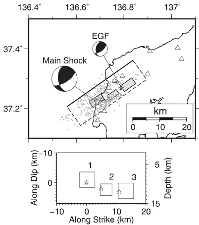
Using the empirical Green’s function (EGF) method (Irikura, 1986; Irikura et al., 1997; Kamae and Irikura, 1998), we construct a source model of the main shock that explains observed broad-band strong ground motions. TheFig. 5. Source model of the 2007 Noto Hanto earthquake estimated using the EGF method. (Upper) Triangles are strong-motion stations. Open and gray rectangles are the assumed fault plane and estimated SMGAs, respectively. Open stars are the epicenter of the main shock and the elemental aftershock used in the modeling, respectively. Focal mechanisms after F-net are also shown. Gray dots are aftershocks occurring on 25 March, 2007. (Lower) Source model. Stars represent the start points of rupture.
EGF method synthesizes waveforms from a target earth-quake (main shock) using those from an elemental small earthquake (aftershock) occurring close to the target earth-quake as Green’s functions. We assume that strong motions are generated from several strong motion generation areas (SMGA) placed on the main-shock fault plane; SMGA usu-ally coincides with the asperity area (Miyakeet al., 2003). The waveform synthesization is based on a rupture propa-gation: the rupture starts from a point on each SMGA with a time delay and radially propagates at an average rupture speed with random time shift (Irikura, 1986).
Table 2. Source parameters of the main shock and aftershock used in EGF modeling.
Event Origin time Epicenter Depth MJ
M0 Area Stress drop
(km) (N m) (km2) (MPa)
Target 07/03/25 09:41 37.221N, 136.686E 10.7 6.9 1.36×10¹⁹∗ — —
Element 07/04/06 15:18 37.267N, 136.790E 11.7 4.3 1.06×10¹⁵† 0.4225 9.38‡
∗F-net.†This study; Fig. 3.‡Brune (1970, 1971).
Table 3. Parameters for strong motion generation areas (SMGAs).
No M0 N∗ C∗ Area Stress drop Rise time Rupture time Slip
†
(N m) (km2) (MPa) (s) (s) (m)
1 2.71×10¹⁸ 8 5 27.0 46.9 0.9 0.0 3.03
2 1.14×10¹⁸ 6 5 15.2 46.9 0.9 2.0 2.27
3 2.17×10¹⁸ 8 4 27.0 37.5 0.9 4.4 2.43
Total 6.02×10¹⁸ 69.3
∗NandCare the ratio of the dimension and stress drop between SMGA and elemental event, respectively.†μ=33 GPa.
Acc.(cm/s )2
EW comp. NS comp.
syn. obs.
Dis.(cm) Vel.(cm/s)
syn. obs.
syn. obs.
EW comp.
NS comp. NS comp. EW comp.
Acc.(cm/s )2 syn. obs.
Dis.(cm) Vel.(cm/s)
syn. obs.
syn. obs.
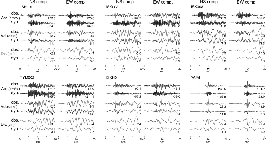
Fig. 6. Comparisons of observed waveforms with synthetic ones calculated using the source model (Fig. 5) for NS and EW components. Each row shows acceleration (top), velocity (middle), and displacement (bottom) waveforms. The numbers on the lower right show a peak amplitude.
S-wave speed. Following Kamaeet al.(1990), different ef-fects of attenuation (Qs) and fmaxbetween the main shock
and elemental event are corrected using the results of spec-tral inversion (Fig. 3(a), (b); ev01 and ev45).
We compare the observed and synthetic data at one KiK-net, one F-KiK-net, and four K-NET stations for the frequency band of 0.3–10 Hz; bore-hole records (at about 200 m depth) are used for the KiK-net station. The aftershock (MJ4.3) occurring at 1518 hours on 6 April is used as an
el-emental event, since this aftershock has a focal mechanism similar to that of the main shock (Fig. 5) and shows simple
S-wave waveform at the stations used in the modeling. The source parameters for the main shock and elemental after-shock are shown in Table 2.
After many trials, we obtain the source model and pa-rameters for SMGAs, as shown in Fig. 5 and Table 3. The rupture speed is estimated to be 2.8 km/s. The observed and
synthetic waveforms show a satisfactory agreement both in shape and amplitude (Fig. 6). The three velocity pulses ob-served at WJM are reproduced in the synthetic waveforms, but amplitudes are underestimated. This may be due to the fact that WJM locates on near the nodal direction of the ele-mental event, and we do not make a correction of a radiation pattern.
4.
Discussion
our model. The slip distribution based on the InSAR data shows, by contrast, a large shallow slip beneath sea region that is not recognized by our data set.
The combined area of SMGA is approximately the half of the value expected by the empirical relationship between the combined area of asperities and seismic moment re-ported by Somervilleet al.(1999). This discrepancy may be due to the dispersion of the empirical relationship; the value of combined area of SMGA is within the spread in values of combined asperity areas used in determining the empirical relationship. However, alternatively, this may be due to the underestimate of the shallow slip beneath the sea region that is not estimated in this study.
Following Dan et al. (2002), we calculate the high-frequency level of acceleration source spectrumAusing the areas and stress drops of SMGA. The A value based on an asperity model (Das and Kostrov, 1986) is expressed as
A=4πβs2
(rnσn)2, wherernandσnare the equiva-lent radius and stress drop of then-th SMGA, respectively. Substituting the parameters in Table 3 into this equation, we obtain A = 3.19×10¹⁹ (N m/s2). After dividing the Avalue by (4πρsβs3R0), we compare the value with the
in-verted source spectrum (Fig. 3; ev01). The high-frequency levels derived from the two analyses are consistent. Hence, the source model corresponds to the asperity model. How-ever, this A value is approximately 2.5 times larger than the empirical relationship for shallow inland and inter-plate earthquakes obtained by Danet al.(2001). Kato and Ikeura (2007) also estimated theAvalue from the inverted source spectrum; their A value is approximately twofold larger than the empirical relationship. These facts indicate that the Noto Hanto earthquake strongly excited high-frequency seismic waves from deep SMGAs.
5.
Conclusions
We applied the spectral inversion method to theS-wave strong motion data from the 2007 Noto Hanto earthquake sequence recorded at temporary and permanent stations in the Noto peninsula. The source spectra of the events show that these events are roughly governed by the scaling re-lation; M0 is proportional to fc−3. We pointed out that a trade-off problem between Qs values and site responses may occur in the case that the extent of hypocenters is much smaller than that of stations in the spectral inversion. We constructed the main-shock source model using the empir-ical Green’s function method. In this model, a combined area of strong motion generation areas was approximately half of the value expected by the empirical relationship. The high-frequency levels of acceleration source spectra
A based on this source model and the spectral inversion were consistent; this indicates that the source model cor-responded to the asperity model. The Avalue was approx-imately 2.5 times larger than the empirical relationship, in-dicating strong excitation of high-frequency seismic waves during the Noto Hanto earthquake.
Acknowledgments. We would like to express our sincere grat-itude to the local government and schools in the Noto peninsula; they kindly allowed us to make observation in their area. We thank
the National Research Institute for Earth Science and Disaster Pre-vention for providing strong-motion data of K-NET, KiK-net, F-net, and moment tensor solutions of F-F-net, and the Japan Meteo-rological Agency for providing hypocentral information and focal mechanisms. This manuscript was greatly improved by construc-tive comments by two anonymous reviewers. Some of the figures in this paper were made using GMT (Wessel and Smith, 1995).
References
Aki, K. and P. G. Richards,Quantitative Seismology. vol. 1, 557 pp, W. H. Freeman and Company, 1980.
Andrews, D. J., Objective determination of source parameters and similar-ity of earthquakes of different size, inEarthquake Source Mechanics, Maurice Ewing Series 6, edited by S. Das, J. Boatwright, and C. H. Scholz, 259–267, Am. Geophys. Union, Washington, D.C., 1986. Boore, D. M. and J. Boatwright, Average body-wave radiation coefficient,
Bull. Seismol. Soc. Am.,74, 1615–1621, 1984.
Brune, N., Tectonic stress and the spectra of seismic shear waves from earthquakes,J. Geophys. Res.,75, 4997–5009, 1970.
Brune, N., Correction,J. Geophys. Res.,76, 5002, 1971.
Dan, K., M. Watanabe, T. Sato, and T. Ishii, Short-period source spectra inferred from variable-slip rupture models and modeling of earthquake faults for strong motion prediction by semi-empirical method,J. Struct. Contr. Eng. AIJ,545, 51–62, 2001 (in Japanese with English abstract). Dan, K., T. Sato, and K. Irikura, Characterizing source model for strong
motion prediction based on asperity model, inProc. 11th Japan Earth-quake Engineering Symposium, 555–560, 2002 (in Japanese with En-glish abstract).
Das, S. and B. V. Kostrov, Fracture of single asperity on a finite fault, in Earthquake Source Mechanics, Maurice Ewing Series, Vol. 6, American Geophys. Union, 91–96, 1986.
Disaster Prevention Research Institute, Kyoto University and Na-tional Research Institute for Earth Science and Disaster Prevention, http://cais.gsi.go.jp/YOCHIREN/JIS/173/image173/018.pdf, 2007. Fire and Disaster Management Agency, http://www.fdma.go.jp/data/
010705141514086149.pdf, 2007.
Geographical Survey Institute, http://cais.gsi.go.jp/YOCHIREN/JIS/173/ image173/016-017.pdf, 2007.
Geographical Survey Japan, Geological Map of Japan 1:200,000 Nanao and Toyama, 1967.
Irikura, K., Prediction of strong acceleration motions using empirical Green’s function,Proc. 7th Japan Earthq. Eng. Symp., 151–156, 1986. Irikura, K., T. Kagawa, and H. Sekiguchi, Revision of the empirical
Green’s function method by Irikura (1986) (program and abstracts), Seism. Soc. Japan 2, B25, 1997 (in Japanese).
Iwata, T. and K. Irikura, Source parameters of the 1983 Japan Sea earth-quake sequence,J. Phys. Earth.,36, 155–184, 1988.
Kamae, K. and K. Irikura, Source model of the 1995 Hyogo-ken Nanbu earthquake and simulation of near-source ground motion,Bull. Seismol. Soc. Am.,88, 400–412, 1998.
Kamae, K., K. Irikura, and Y. Fukuchi, Prediction of strong ground motion forM7 earthquake using regional scaling relations of source param-eters,J. Struct. Constr. Eng, AIJ,416, 57–70, 1990 (in Japanese with English abstract).
Kato, K. and T. Ikeura, Source, path, and site effects of the Noto Hanto Earthquake in 2007; Preliminary results based on K-NET and KiK-net records,Japan Geoscience Union Joint Meet., Z255-P036, 2007. Maeda, T. and T. Sasatani, Two-layerQs structure of the slab near the
southern Kurile trench,Earth Planets Space,58, 543–553, 2006. Miyake, H., T. Iwata, and K. Irikura, Source characterization for broadband
ground-motion simulation: kinematic heterogeneous source model and strong motion generation area,Bull. Seismol. Soc. Am.,93, 2531–2545, 2003.
Somerville, P., K. Irikura, R. Graves, S. Sawada, D. Wald, N. Abrahamson, Y. Iwasaki, T. Kagawa, N. Smith, and A. Kowada, Characterizing crustal earthquake slip models for the prediction of strong ground motion, Seismol. Res. Lett.,70, 59–80, 1999.
Wessel, P. and W. H. Smith, New version of the Generic Mapping Tools released,EOS Trans. AGU, 329, 1995.