Rupture process during the 2007 Noto Hanto earthquake (MJMA 6 9) and strong motion simulation in the source region

(1)

Rupture process during the 2007 Noto Hanto earthquake (

M

_JMA

6.9) and

strong-motion simulation in the source region

Yoshiaki Shiba

Central Research Institute of Electric Power Industry, 1646 Abiko, Abiko-shi, Chiba 270-1194, Japan

(Received July 2, 2007; Revised May 8, 2008; Accepted July 1, 2008; Online published November 7, 2008)

The source rupture process during the 2007 Noto Hanto earthquake is inferred using a broadband waveform inversion technique based on the empirical Green’s function and the simulated annealing. The spatio-temporal distributions of the moment density and rise time on the fault are estimated from displacement motions in the frequency range from 0.1 to 2 Hz, and effective stress distribution is derived from the velocity motions in the frequency range up to 5 Hz. Results from the displacement inversion indicate that the seismic moment is mainly

released from a single asperity with an area of 10×10 km2_{, and total moment release is estimated to be about}

1.3×1019_{N m. The velocity inversion shows that the high effective stress area distributes on and around the}

asperity, in particular at the deep periphery of it. The broadband strong motions determined using the conventional source model composed of only the moment distribution are compared with those calculated by considering both moment and effective stress separately. The ﬁt between observed acceleration motions and synthetic ones from both source models are generally good in the frequency range up to 10 Hz, and no evident difference is recognized.

Key words:Rupture process, waveform inversion, strong ground motion, simulated annealing, empirical Green’s

function.

1. Introduction

The Noto-Hanto earthquake (MJMA6.9) occurred on 25

March 2007 on the Noto peninsula, Ishikawa prefecture on the Coast of the Japan Sea. Most of the main shock fault lies beneath the inland area, and some towns suffered se-vere damages. Since tens of strong-motion observation sta-tions are distributed on and around the source area, installed by the National Research Institute for Earth Science and Disaster Prevention, called K-NET (Kinoshita, 1998) and

KiK-net (Aoiet al., 2000), and by the Japan

Meteorologi-cal Agency (JMA), this event is an appropriate case for in-vestigating the detailed source rupture process generating strong motions, though the station coverage might not be satisfactory.

In this article I apply the source inversion scheme com-posed of the empirical Green’s function method and sim-ulated annealing (Shiba and Irikura, 2005) to broadband strong-motion data from the 2007 Noto Hanto earthquake and separately estimate the spatio-temporal distributions of the seismic moment and effective stress on the fault. Wave-form ﬁtting for the velocity motions in the frequency range up to 5 Hz is performed in order to directly infer the detailed source process radiating the high-frequency strong motions from the observed data. To represent the real rupture pro-cess, effective stress is added to the independent source pa-rameters describing a variation of the slip velocity function on the fault, together with the seismic moment, rise time, and rupture time. I then compare the synthetic ground

mo-Copyright cThe Society of Geomagnetism and Earth, Planetary and Space Sci-ences (SGEPSS); The Seismological Society of Japan; The Volcanological Society of Japan; The Geodetic Society of Japan; The Japanese Society for Planetary Sci-ences; TERRAPUB.

tions in the broadband frequency range (0.1 to 10 Hz) cal-culated from the source model estimated by proposed in-version method and those determined by the conventional method to reveal important parameters for predicting broad-band strong ground motions.

2. Inversion Method

The inversion scheme used in this study is principally based on the method proposed by Shiba and Irikura (2005). This method is composed of the very fast simulated an-nealing (VFSA), which is one of the heuristic search algo-rithms used to statistically ﬁnd the best global solution of a nonlinear nonconvex (multimodal) problem (Ingber, 1989;

Kirkpatricket al., 1983), and the empirical Green’s

func-tion method (EGFM; Irikura, 1986) as a forward process to calculate synthetic ground motions. In order to exam-ine the detailed source process radiating broadband, par-ticularly high-frequency ground motions, I adopt two-step inversion scheme, in which displacement motions are first inverted to search the moment and rise time distributions with rupture times, and then velocity motions are compared with synthetic motions to find the effective stress distribu-tion with fixed rise time and variable moment density. For the shape of the slip velocity function (exactly a filter func-tion in the EGFM) on the fault, the displacement inversion employs a boxcar function with the height proportional to the seismic moment and the duration equivalent to the rise time. In contrast, the velocity inversion uses a combination of a delta function proportional to the effective stress and the boxcar function to satisfy the similarity law of source

spectra, this is called theω-square model (Aki, 1967) to the

higher frequency range. The seismic moment and rise time

(2)

Main Shock

2007/3/28 08:08 ISK001 ISK002

ISK003

ISK004

ISK005

ISK006

ISK007

ISK008

ISKH01

ISKH02

Central Japan

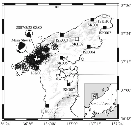
Fig. 1. Location map showing the strong-motion stations, initial fault model of the main shock, and epicenters of aftershocks. Solid and open squares show the K-NET and the KiK-net stations, respectively. Star symbols indicate epicenters of the main shock and the element event used as the empirical Green’s function. Circles indicate the epicenters of aftershocks within 24 h after the main shock, and their sizes vary with the magnitude.

control low-frequency motions, while the effective stress and the variation of rupture times are strongly related to the high-frequency radiation. Therefore, the seismic moment and rise time distribution are estimated from the displace-ment motions before the search of effective stress variation by ﬁtting the high-frequency velocity waveforms to ensure the stability of inversion results.

In this study I adopt some modiﬁcations or improvements to the proposed method of Shiba and Irikura (2005). A spa-tial smoothing constraint for all search parameters except rupture time is imposed to suppress the instability of solu-tions following Yoshida and Koketsu (1990) such as,

∇2_Xm

,n =Xm+1,n+Xm,n+1−4Xm,n+Xm−1,n+Xm,n−1

=0 (1)

whereXm_,nis a search parameter at themn-th subfault, and

∇2 _{is a discrete Laplacian operator. Suitable weights for}

the smoothing constraint are determined through Akaike’s Bayesian Information Criterion (ABIC; Akaike, 1980). Rupture time variation obeys only the causality; that is, a subfault does not fail until its neighbor nearest to the rup-ture initiation point has failed (Ihml´e, 1996). Furthermore, in the velocity inversion, the rupture time at each subfault is searched from a set of samples repeatedly accepted in the displacement inversion below the “critical temperature” during the cooling process of the VFSA. Such a procedure implies that the marginal a posteriori distribution of sam-pled parameters after the displacement inversion is utilized as a priori distribution for the velocity inversion. We then can make use of both stability in the displacement inversion and high resolution in the velocity inversion to estimate the detailed rupture propagation on the fault (Shiba, 2006).

Table 1. Search areas of model parameters used in the displacement inversion. vris rupture velocity andβis the S-wave velocity in the source area.

Moment ratio 0.0–5.0

Rise time (s) 0.0–3.0

vr/β 0.6–1.0

Table 2. Search areas of model parameters used in the velocity inversion.

Effective stress ratio 0.0–10.0

Amplitude ratio of boxcar func. 0.0–5.0

vr/β 0.6–1.0

3. Data and Initial Fault Model

Strong-motion records from ten stations, which are eight K-NET and two KiK-net surface stations, are used for the inversion. Figure 1 shows the location map of the stations along with the assumed fault plane of the main shock, the epicenter of the element event used for an empirical Green’s function in the inversion analysis, and other aftershocks oc-curring within 24 h after the main shock. The hypocen-ter locations of these events are dehypocen-termined using the JMA uniﬁed catalog. In the initial fault model the size covering

the aftershock distribution is assumed to be 36×22 km2

(Fig. 1). I assume N58◦E for the strike angle and 66◦ for

the dip angle following the moment tensor solution of F-net

(Fukuyamaet al., 1998). The empirical Green’s function

chosen in this study is an aftershock of MJMA4.9, which

occurred on 28 March 2007 at 08:08 near the hypocenter of the main shock (and center of the assumed fault plane). The

main-shock fault is divided into 19×11 subfaults 1.9 km

long and wide. The size of the subfault, which is equiva-lent to the source area of the element event (the empirical Green’s function), is determined by taking a spectral ratio of the main shock to the element event at each station (Miyake

et al., 2003). The corner frequency of the element event is derived from the average spectral ratio, and the equiva-lent source radius of the element event is estimated from the Brune’s source model (Brune, 1970, 1971).

The observed acceleration records are numerically inte-grated to obtain data of the displacement and velocity mo-tions, and they are band-pass-ﬁltered from 0.1 to 2 Hz for the displacement inversion and to 5 Hz for the velocity in-version. The lower limit of the ﬁlter is determined accord-ing to the signal-to-noise ratio of the Fourier spectra for the

observed element event. TheS-wave portions of two

hori-zontal ground motions are used for the inversion.

4. Inversion Results

4.1 Control parameters for inversion procedure

Tables 1 and 2 show the search areas of model param-eters used in the displacement and the velocity inversions, respectively. In the inversion scheme used in this study, the search parameters, such as the moment density and the ef-fective stress, are represented as the ratio to those of the ele-ment event. The search area of the rupture time is described

as the variation of normalized rupture velocity with theS

(3)

2 s.

2 s. 4 s.

6 s.

8 s.

8 s. 8 s.

10 s

dip direction (km)

strike direction (km)

Moment Density from D (*1016_Nm/km2₎

0 1 2 3 4 5 6 7 8 9 10

2 s. 4 s.

6 s.

8 s. 8 s.

10

s 10

s.

dip direction (km)

Moment Density from V (*1016_Nm/km2₎

0 1 2 3 4 5 6 7 8 9 10

2 s. 4 s.

6 s.

8 s. 8 s.

10 s

10 s.

dip direction (km)

0 2 4 6 8 10 12 14 16 18 20

Effective Stress (MPa)

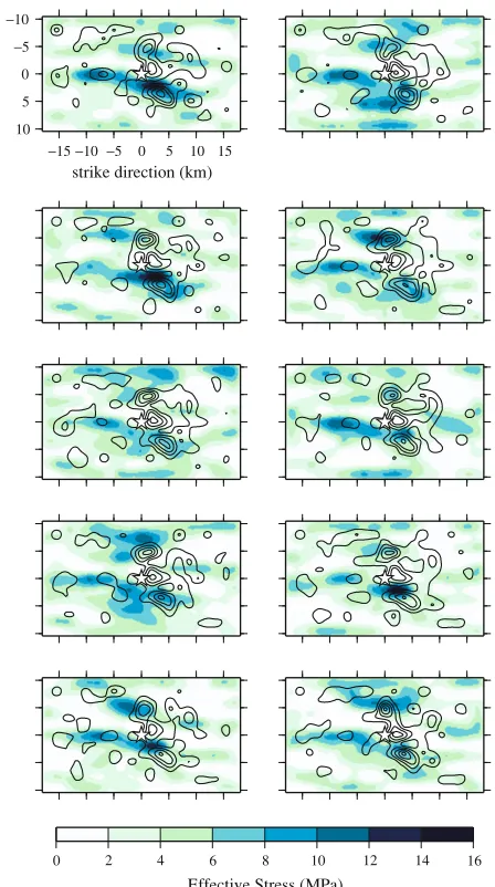
Fig. 2. Optimal source models obtained from the VFSA inversions. Upper figure shows the moment distribution derived from the displacement inversion. Middle figure and lower figure show the moment and the effective stress distributions from the velocity inversion, respectively. Contour at each figure displays the rupture time distribution.

2005),

M0/m0=C1+C2·(N−1) , (2)

where M0 andm0 are the moment of the main shock and

the element event, respectively.C1is the effective stress

ra-tio and it implies the amplitude of the delta funcra-tion in the context of the ﬁlter function for the formulation of the

em-pirical Green’s function method (Irikura, 1986).C2implies

the amplitude of the following boxcar function (or the

expo-nentially decaying function) in the EGFM. Nis the scaling

parameter and is approximately equivalent to the average rise time ratio of the main shock to the element event.

Since the focal mechanism of the element event is dif-ferent from that of the main shock, as shown in Fig. 1, I

follow the method of Kamaeet al.(1990) to correct the

ra-diation pattern so as to be smoothed gradually toward the high-frequency range. In this study, the radiation coefﬁ-cient obeys the theoretical value in the frequency range less than 0.5 Hz, and reaches the azimuthal average at 5 Hz as

suggested in Kamaeet al.(1990). Radiation pattern is also

averaged for takeoff angles in the range from 120◦to 180◦

(Boore and Boatwright, 1984).

dip direction (km)

0 2 4 6 8 10 12 14 16

Effective Stress (MPa)

Fig. 3. Source models mapping both the moment and the effective stress distributions from 10 inversion attempts with different initial random numbers. The contour lines show the moment density and are drawn for every 2×1016N m/km2. Blue images represent the effective stress.

The cooling schedule during the simulated annealing is written as follows (Ingber, 1989),

T(k)=T0exp

−qkp, (3)

whereT is the “temperature” decreasing exponentially in

the cooling timek, and it controls the probability to accept

the change increasing misﬁt. T0 is an initial temperature,

andpandqare appropriate constants adjusting the cooling

speed of the system, which are determined through the test runs (preliminary inversions).

4.2 Obtained optimal solutions

(4)

NS

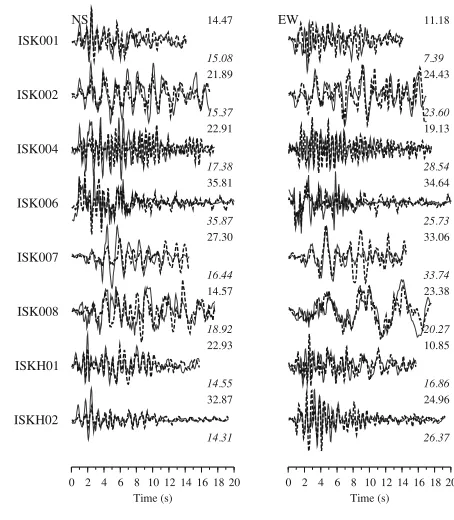
Fig. 4. Comparison of synthetic and observed displacement waveforms. Solid lines show the observed waveforms and broken lines denote syn-thetic ones. Numbers above the waveforms are the peak values of ob-served motions and those below the waveforms are the peak values of synthetics, respectively.

possibility of the nonlinearity effect during the main shock. The seismic moment is released mainly from the relatively small area of 10 km long and wide in the northeast direc-tion derived from the rupture starting point (a star in the ﬁg-ure). The moment and the rupture time distributions derived from the velocity inversion are very similar to that from the displacement inversion, in spite of different frequency-band and shapes of ﬁlter functions assumed in the forward process. The totally released moment is estimated to be

about 1.3×1019_{N m. The rupture velocity on the fault is}

rather constant except for the area just above the hypocen-ter, where the rupture propagation is slightly accelerated.

In contrast, the distribution of the effective stress seems to be different from that of the moment. We see the high effective stress area not only at the northeastern direction, but also in the deeper part from the hypocenter. Figure 3 shows the 10 inversion results plotting both the moment and the effective stress distributions. Though there are some differences among the obtained source models depending on the initial random number in the inversion, we can see common characteristics that the high effective stress area distributes on the shallow asperity and the periphery of the deep asperity. The deeper area of high effective stress might work as the barrier that terminates the growth of an asperity. Figures 4 and 5 show the comparison between the syn-thetic motions from the best inversion solution and the

ob-NS

Fig. 5. Comparison of synthetic and observed velocity waveforms. Solid lines show the observed waveforms and broken lines denote synthetic ones. Numbers above the waveforms are the peak values of observed motions and those below the waveforms are the peak values of syn-thetics, respectively. ISK003 and ISK005 are not used in the velocity inversion.

served motions for the displacement and the velocity in-versions, respectively. The ﬁts between them are generally good for both inversions.

5. Estimation of Broadband Strong Motions

The aim of the inversion scheme employed here is to demonstrate that it is possible to evaluate broadband strong motions directly from the source inversion results without any assumptions to connect the high-frequency radiation in-tensity and the moment distribution on the seismic source. By estimating the seismic moment and the effective stress on the fault separately, it is possible to invert the velocity motions in the frequency range up to 5 Hz successfully. Here I calculate the acceleration motions to 10 Hz, which are of engineering interest for estimating input ground mo-tions in the seismic design, by using the optimal source models estimated from the velocity inversion along with those from the displacement inversion. The source model from the displacement inversion in this study is interpreted as the conventional model described with only the moment distribution. Therefore, the advantage of employing this proposed inversion method is veriﬁed by comparing the synthetic broadband motions from both inversions with the observed motions.

(5)

ISK001 Acceleration (cm/s/s)

Obs.

158.74

Velocity (cm/s)

15.02

D_Syn.

196.35 11.63

V_Syn.

163.96 14.18

ISK002

170.81 22.18

135.11 27.70

162.67 26.76

ISK003

447.01 38.37

1414.42 79.12

1336.19 72.93

ISK004

453.70 23.17

306.86 21.26

267.59 21.26

ISK005

401.37 35.01

874.53 70.95

1004.95 66.93

0 10 20 30

Time (s)

0 10 20 30

Time (s)

ISK006 Acceleration (cm/s/s)

549.70

Velocity (cm/s)

36.29

569.75 42.85

688.71 33.75

ISK007

198.62 26.89

191.28 19.55

201.88 19.03

ISK008

233.20 16.44

214.11 25.82

190.84 17.81

ISKH01

355.22 23.07

134.49 14.26

179.95 14.35

ISKH02

256.96 33.19

182.79 13.79

200.46 16.76

0 10 20 30

Time (s)

0 10 20 30

Time (s)

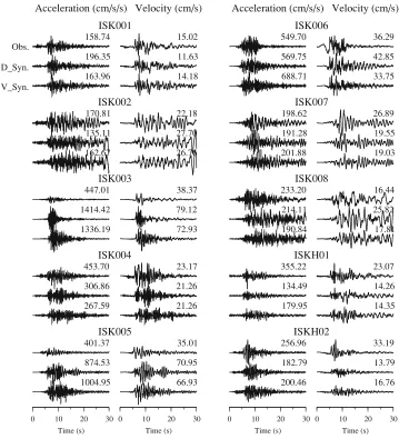
Fig. 6. Comparison of synthetic and observed motions on the NS component in the broadband frequency range from 0.1 to 10 Hz. At each station the top trace shows the observed waveform, while the middle and bottom traces indicate the synthetic motions from the displacement inversion and the velocity inversion respectively. Numbers above the waveforms are the peak values.

due to the nonlinearity effect of the sedimentary soils, as suggested earlier. For other stations, observed motions are reproduced generally well by using both inversion methods. Figure 7 shows the pseudo velocity response spectra for the observed and synthetic motions. As seen in Figs. 6 and 7, in this case, an obvious advantage over the source model based on the velocity inversion to that from conventional method cannot be shown. If there were to be a strong-motion sta-tion just near the separately existing area of higher effective stress, the difference between them might become clear. On the other hand, the strong-motion prediction based on the conventional inversion using low-frequency motions is still valid under the condition of the station distribution used in this study relative to the dimensions of the seismic source.

6. Discussion and Conclusions

In this article I applied the inversion method using very fast simulated annealing with the empirical Green’s func-tion method to the strong mofunc-tion records from the 2007 Noto Hanto earthquake in order to obtain the rupture pro-cess radiating broadband ground motions. The inversion results indicate that the effective stress shows spatial

dis-tributions partly different from that of the seismic moment, suggesting barrier-like behavior which decelerates or termi-nates the growth of an asperity. However, the source model using the moment and effective stress variation separately estimated from the velocity inversion do not improve the synthetic acceleration motions in the frequency range up to 10 Hz and show almost same accuracy as the conventional low-frequency inversion.

Several researchers have estimated the slip distributions for this event through the inversion technique with strong-motion data (e.g. Horikawa, 2007; Iwata and Asano, 2007). Their source models commonly have one main asperity on the area including the hypocenter, which is consistent with my result. However, the asperity in the other many models is located on the shallower area from the hypocenter, while my model shows the asperity also extends to the deep direc-tion.

(6)

0.1 1 10 100

Pseudo Velocity (cm/s)

0.1 1 10

Fig. 7. Comparison of pseudo velocity response spectra (h = 5%) for synthetic and observed motions on the NS component. Solid lines show the observed motions. Gray lines and broken lines are the synthetic motions from the displacement and the velocity inversions, respectively.

evaluation and/or the prediction of strong ground motions (e.g. Irikura, 2004). The idea of the source characteriza-tion is based on the reports that the asperity estimated from the low-frequency inversion corresponds to the strong

mo-tion generamo-tion area (Miyake et al., 2003). The results

obtained from this study suggest that the observed strong motions are well reproduced using the source model com-posed of only the moment distribution, though the effec-tive stress shows the different distribution from the moment.

Future works should be focused on the application of the broadband waveform inversion to the larger event such that the near-source strong motion records (just above the fault plane) are obtained at several points.

Acknowledgments. I would like to thank the K-NET, KiK-net, and F-net operated by the National Research Institute for Earth Science and Disaster Prevention (NIED) for providing the strong-motions records and moment tensor solutions. I thank the EPS reviewers and editor for their helpful comments. Figures were prepared with the Generic Mapping Tools (Wessel and Smith, 1998).

References

Akaike, H., Likelihood and the Bayes procedure, in Bayesian Statics, University Press, Valencia, Spain, 1980.

Aki, K., Scaling law of seismic spectrum,J. Geophys. Res.,72, 1217–1231, 1967.

Aoi, S., K. Obara, S. Hori, K. Kasahara, and Y. Okada, New strong-motion observation network: KiK-net,Eos Trans. AGU, 329, 2000.

Boore, D. and J. Boatwright, Average body-wave radiation coefﬁcients, Bull. Seismol. Soc. Am.,74, 1615–1621, 1984.

Brune, J., Tectonic Stress and the Spectra of Seismic Shear Waves from Earthquakes,J. Geophys. Res.,75, 4997–5009, 1970.

Brune, J., Correction,J. Geophys. Res.,76, 5002, 1971.

Fukuyama, E., M. Ishida, D. S. Dreger, and H. Kawai, Automated seismic moment tensor determination by using on-line broadband waveforms, Zisin 2 (J. Seismol. Soc. Jpn.),51, 149–156, 1998 (in Japanese with English abstract).

Horikawa, H., Source rupture process of 2007 Noto-Hanto Earthquake, http://unit.aist.go.jp/actfault/katsudo/jishin/notohanto/hakaikatei2.html, 2007 (in Japanese).

Ihml´e, P. F., Monte Carlo slip inversion in the frequency domain: Appli-cation to the 1992 Nicaragua slow earthquake,Geophys. Res. Lett.,9, 913–916, 1996.

Ingber, L., Very fast simulated re-annealing,Mathl. Comput. Modelling, 12, 967–973, 1989.

Irikura, K., Prediction of strong acceleration motions using empirical Green’s function,Proc. 7th Jpn. Conf. Earthq. Eng., 151–156, 1986. Irikura, K., Recipe for predicting strong ground motion from future large

earthquake,Ann. Disas. Prev. Res. Inst., Kyoto Univ.,47, A, 2004 (in Japanese with English abstract).

Iwata, T. and K. Asano, Source process characteristics of the 2007 Noto-Hanto earthquake,The 35th Symposium of Earthquake Ground Motion, 7–12, 2007 (in Japanese with English abstract).

Kamae, K., K. Irikura, and Y. Fukuchi, Prediction of strong ground motion for M7 earthquake using regional scaling relations of source parame-ters,J. Struct. Constr. Engng, AIJ,416, 57–70, 1990 (in Japanese with English abstract).

Kinoshita, S., Kyoshin net (K-NET),Seismol. Res. Lett.,69, 309–332, 1998.

Kirkpatrick, S., C. D. Gelatt, and M. P. Vecchi, Optimization by simulated annealing,Science,220, 671–680, 1983.

Miyake, H., T. Iwata, and K. Irikura, Source characterization for broadband ground-motion simulation: Kinematic heterogeneous source model and strong motion generation area,Bull. Seismol. Soc. Am.,93, 2531–2545, 2003.

Shiba, Y. and K. Irikura, Rupture process by waveform inversion us-ing simulated annealus-ing and simulation of broadband ground motions, Earth Planets Space,57, 571–590, 2005.

Shiba, Y., Improvement of inversion technique with simulated annealing to estimate more accurate and well-resolved source parameters, Pro-gramme and Abstracts, Seismol. Soc. Jpn., 2, P068, 2006 (in Japanese). Yoshida, S. and K. Koketsu, Simultaneous inversion of waveform and geodetic data for rupture process of the 1984 Naganoken-Seibu, Japan, earthquake,Geophys. J. Int.,103, 355–362, 1990.

Wessel, P. and W. H. F. Smith, New, improved version of Generic Mapping Tools released,Eos Trans. AGU,79, 579, 1998.